A Multi-sensory Stimuli Computation Method for Complex Robot
Behavior Generation
Younes Raoui and El Houssine Bouyakhf
Laboratory of Computer Sciences, Applied Mathematics, Artificial Intelligence and Pattern Recognition,
Physics Department, Faculty of Sciences, Mohamed V University, 4 Ibn Battouta Street, Rabat, Morocco
Keywords:
Robot Navigation, Neural Fields, Global Visual Descriptor, Robot Behavior, Extended Kalman Filter.
Abstract:
In this paper we present a method for obstacle avoidance which uses the neural field technique to learn the
different actions of the robot. The perception is used based on monocular camera which allows us to have
a 2D representation of a scene. Besides, we describe this scene using visual global descriptor called GIST.
In order to enhance the quality of the perception, we use laser range data through laser range finder sensor.
Having these two observations, GIST and range data, we fuse them using an addition. We show that the fusion
data gives better quality when comparing the estimated position of the robot and the ground truth. Since we
are using the paradigm learning-test, when the robot acquires data, it uses it as stimuli for the neural field in
order to deduce the best action among the four basic ones (right, left, frontward, backward). The navigation is
metric so we use Extended Kalman Filter in order to update the robot position using again the combination of
GIST and range data.
1 INTRODUCTION
To avoid obstacles is considered nowadays very im-
portant behaviour in the robotic community. It is
often relied to localization and mapping since the
robot has to move in its environment. Therefore, the
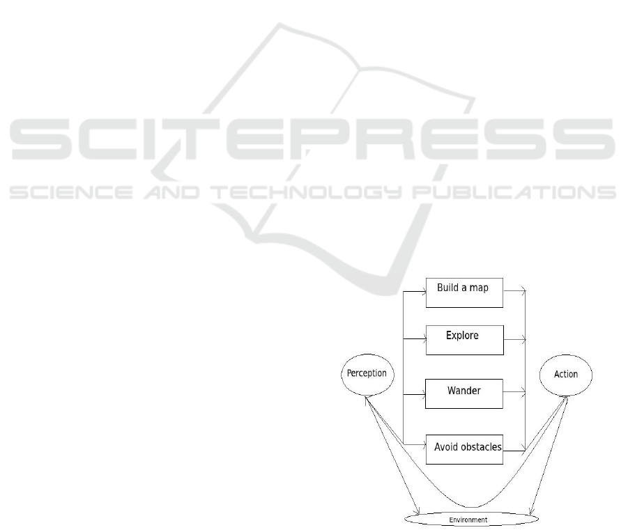
robot has to satisfy the three blocks of the reactive
paradigm 1. Up to now, methods called soft com-
puting such as fuzzy logic and reinforcement learn-
ing have been widely used in the literature. However,
the neural approach inspired from the human biology
is considered an alternative to the cited methods be-
cause it is simpler and more efficient. We propose in
this work a novel method using the neural fields(Yan
et al., 2012)for behaviour generation. The neural field
method is the continuous version of the neural net-
works, well known in the robotic community. The
neural fields have entries called stimuli and outputs
called actions. Although the use of a certain single
stimulus can trigger correct actions to avoid obstacles,
it shows some drawbacks such as lack of information
quantity. For example, if a robot moves in an outdoor
environment, the use of laser signal is not efficient at
all since this the distance and the orientation of the
reflected signal are affected by natural noise. Con-
sequently, we propose in this work to deal with the
problem of the perception of the robot environment.
Figure 1: Reactive Paradigm.
We propose to fuse data sensors from cameras and
laser range finders. We use global features to repre-
sent globally the contain of an image. Secondly, we
will fuse these measures of luminance with the laser
data observations (distance and orientation) given that
we will use the range and bearing model to model the
response of the laser range finders.
139
Raoui Y. and Bouyakhf E..
A Multi-sensory Stimuli Computation Method for Complex Robot Behavior Generation.
DOI: 10.5220/0005528301390145
In Proceedings of the 12th International Conference on Informatics in Control, Automation and Robotics (ICINCO-2015), pages 139-145
ISBN: 978-989-758-122-9
Copyright
c
2015 SCITEPRESS (Science and Technology Publications, Lda.)

2 RELATED WORKS
In (Yan et al., 2012), a neural architecture for learn-
ing new navigation strategies of a robot is proposed
based of the observation of human’s movements. In
(Y.Sandamirskaya et al., 2011), a new architecture
for behavioural organization of an agent is proposed.
Since it receives data from sensors and the environ-
ment of the robot, the behaviour is determined with
actions.Also a theoretical formula based on Bayes
rules and neural field is given. The work of (P.Cisek,
2006) is for major importance in the robot grasping
field. Indeed, it gives a theory for object grasping
based on the strategies used for animals to decide
which object to reach and how to do the planning
of the movement. Because these processes stimulate
the same brain regions, (C.Crick, 2010) developed a
model which allow to fix and to plan through some pa-
rameters of the movement. In the area of navigation,
(M.Milford and G.Wyeth, 2010) has given another
view of SLAM by using a biological approach. This
method allows the robot to localize it self in a variable
large environment. (Maja, 1992) proposed a method
which synthesises an artificial robot behaviour of the
robot. This life like strategy should be robust, repeat-
able and adaptive. Concerning the global descriptor
used to characterize images, many works are done. A
survey is given in (Y.Raoui et al., 2010).
3 LOCALIZATION WITH EKF
USING LASER RANGE FINDER
In this section, we are interested to robot localization
in a structured environment using the probabilistic ap-
proach(Y.Raoui et al., 2011). This approach has in-
duced a revolution in robotics since Thrun introduced
it in 95. Indeed, it takes into account the uncertainty in
the movement of the robot. This uncertainty is caused
with many factors like ”slippage, bumping”. Through
the fusion of sensor and motion model, th robot can
correct its positions. In the figure ”ground”, we show
the positions where the robot should be. These states
are of crucial importance because all the steps of fil-
tering are depending on it. The robot has to compare
its noisy position with the ground truth.
3.1 Prediction of the Position
The most important thing to consider in the prediction
phase is the motion model or the model of displace-
ment of the robot. It should be in fact determined
with a probabilistic way, in order to move the mobile
robot. Let’s have the following probability with rely
the robot position from x
t
tox
t+1
with an action u.
p(x
t+1
/x
t
,u)
In order to implement this equation, we use the pre-
diction step of the Kalman filter:
X
t+1
= A.X
t
+ B ∗ u
In this implementation, we consider the robot state
as a couple of the robot mean position and the co-
variance. This distribution will evolute until the robot
ends its path.
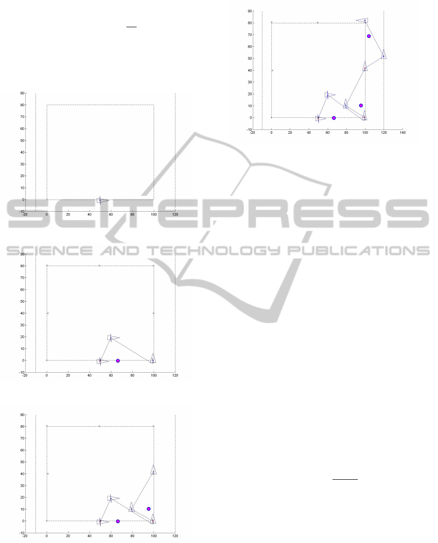
The figure 1 shows the movement of the robot in
a structured environment. We consider the state of
the robot represented with (x,y,θ) which simplifies
its estimation. For more complete formulation, we
should integer Euler angles. As shown in the figure,
the robot positions are affected with error which dis-
able the robot to close the loop. This ability is im-
portant for both indoor and outdoor environments. At
the same time, the ellipse of uncertainty grows also
because the predicted covariance is growing. Thus,
a step of correction must be included so as we can
reduce this ellipse of uncertainty, in other words de-
crease the values of the diagonal of the covariance
matrix.
3.2 Correction of the Position
To update the position of the robot we use the ob-
servation computed from Laser range data and GIST
descriptor both as done for the stimuli. Let us have
the function z(x) where x is the robot position and z
is the observation.
We have H =
dz
dx
is the Jacobian which will allow
us to update the robot metrical position using the fol-
lowing equations:
Q
t
= (
σ
2
r
0
0 σ
2
r
)
Where σ
r
is the standard deviation of the robot
motion.
S
t
= H
t
∑
t
∗ H
T
t
+ Q
t
S
t
is the covariance on the predicted measure, which
the noise could be from the monocular camera or the
Laser range finder.
K
t
=
∑
t
∗ H
T
t
∗ S
−1
t
K
t
is the Kalman gain. Q is the error on the robot
position.
The equation of the update of the robot position is:
X
t+1
= X
t
+ K
t
∗ (z
t
− ˆz
t
)
ICINCO2015-12thInternationalConferenceonInformaticsinControl,AutomationandRobotics
140
The covariance of the update is:
∑
t
= (I − K
t
∗ H
t
)
∑
t
and (z
t
− ˆz
t
) expresses the data association for local-
ization, in other words the difference between the ob-
servation and the prediction of the measure.
Figure 2.
Figure 3.
Figure 4.
Figure 5: Figures 2,3,4 and 5 represent ground truth with
red points, predicted positions with blue points and esti-
mated positions with triangle.
4 NEURAL FIELDS
4.1 Behavior Control with Neural Fields
based on Laser Range Finders
The main actions of the mobile robot are moving for-
ward, backward, left or right. Indeed, the neural fields
are used to encode the direction of the robot by mean
of their peaks. The stimulus are supposed to be the
sensory data which are provided by the robot sensors.
This method implies the use of the sensing-action
paradigm without using any planning task. Therefore,
the neural field is expressed by the one-dimensional
equation:
τ.u(ϕ,t) = −u(ϕ,t) + s(ϕ,t) + h+
Z
w(ϕ,ϕ
0
). f (u(ϕ
0
,t))dϕ
0
where T ¿ 0 defines the time-scale of the field, u is the
field excitation at the position neuron. The temporal
derivative of the excitation is defined by:
u
.
(ϕ,t) =
u(ϕ,t)
dt
The stimuli represents the input of the field at a certain
position and at time t. Depending on the stimuli, the
equation can have different solutions:
• 0-solution, if u(ϕ) < 0
• infinite solution, if u(ϕ) > 0
• a-solution, if there is localized excitation from a
position a
1
to a position a
2
. This solution is also
called a single-peak or mono-modal solution.
AMulti-sensoryStimuliComputationMethodforComplexRobotBehaviorGeneration
141
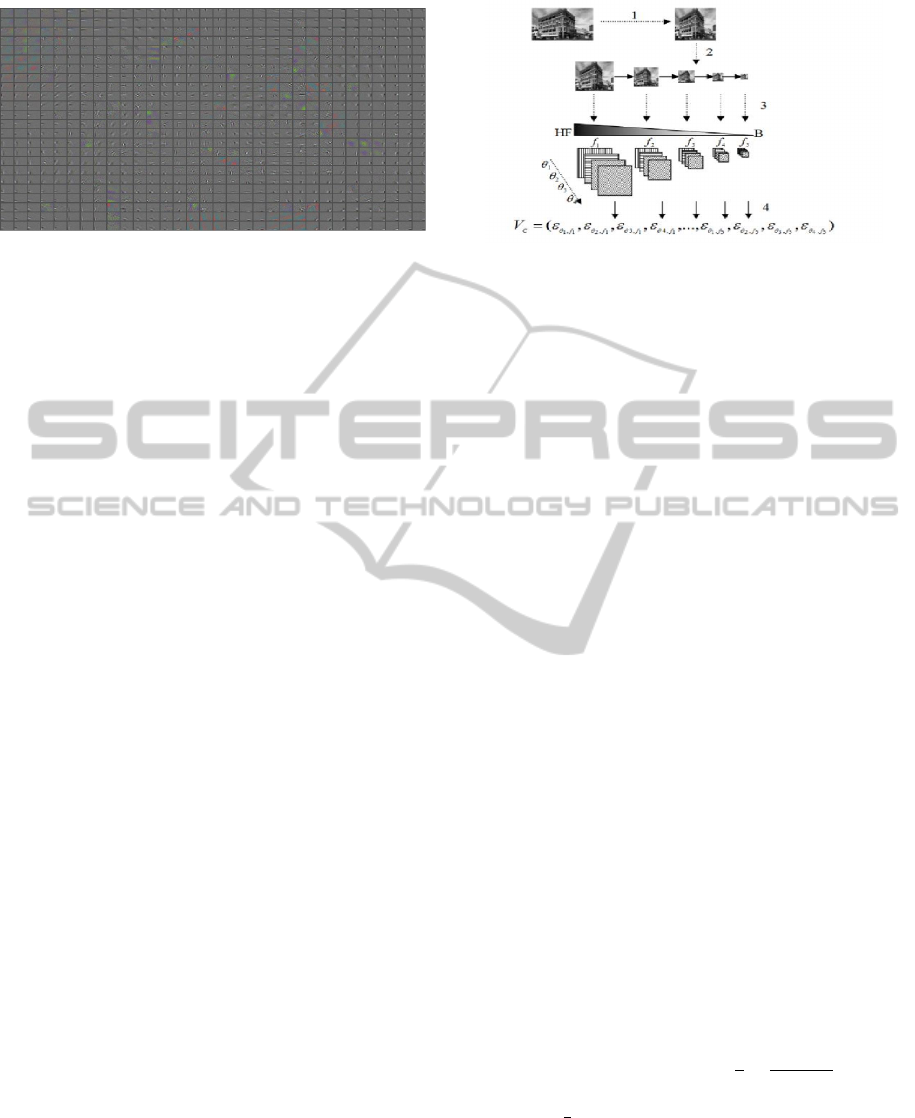
Figure 6: Receptive neural field.
The neural fields can control the robot’s planar move-
ments with:
• Target-Acquisition: moving towards a given tar-
get point.
• Obstacle Avoidance: moving while avoiding ob-
stacles.
• Corridor Following: moving along corridors in
the absence of obstacles.
• Door Passing: passing a door to traverse between
two rooms, from a corridor to a room, or vice
versa.
4.1.1 Control Design
The behavioural variable is taken as the robot’s head-
ing ϕ relative to a world fixed reference. Then, the
neural field has to encode angles from −pi to +π. The
global inhibition allows only one localized peak on
the field. After the stabilization of the field, the most
activated neuron decodes the direction to be executed
by a robot.
Field of Stimuli
The neural field needs some necessary informations
(stimuli). The stimulus is determined according to
some stimulus functions. These functions describe
the target direction, the direction to obstacles. A novel
feature of our approach is the use of vision and laser
range informations as stimuli. We will propose a
model of sensor with noise which will correct the po-
sition of the robot.
Dynamics of Speed
In a free obstacle situation, the robot moves with its
maximum speed Vmax, and slows down when it ap-
proaches a target. This velocity dynamics can be cho-
sen as:
V
T
(t) = V
max
(1 − exp
σ
v
.d
T
)
where σ
v
is a positive constant tuned in a relation with
the acceleration capability of the robot. dT represents
the distance between the robot and the target at time
t.
Figure 7: An explivative scheme of the GIST descriptor.
5 METHODS
We present a novel method, based on Dynamic Neu-
ral Fields, for multi-sensory fusion of visual and laser
data. Wo compute the GIST global visual features
(Oliva and A.Torralba, 2001) for images which we
fuse with range and bearing data measured with laser
range finders.
5.1 GIST Descriptor
Visual global features are 1D vectors that allows to
describe and index images. GIST reduces the dimen-
sion of such features. First the images are decom-
posed into small images which size are 32*32 and
128*128. Second, they are smoothed with Gabor fil-
ters having n
θ
and n
σ
scales. Third, the obtained fil-
tered images are divided on M*N regions and trans-
formed on a vector.
5.2 Stimuli Computation
We compute our stimuli using monocular camera and
laser range sensors as showing in the figure 6 . The
neural fields are machine learning methods which are
better that the other non-linear methods such as SVM
and Mixture of Gaussians.
The equation of Amari (Amari, 1977) has as un-
known variable u(φ,t) which solution is given in the
following equation(see 8):
u(φ,t) = aexp(−(1 − α.K)
t
τ
+
1 − α
1 − α.K
.S
where α =
1
2
et τ = 10.
and
K =
N
∑
φ=1
ω(|φ − φ
0
|) ∗ H(φ) (1)
H(φ) is the heaveside function.
ICINCO2015-12thInternationalConferenceonInformaticsinControl,AutomationandRobotics
142
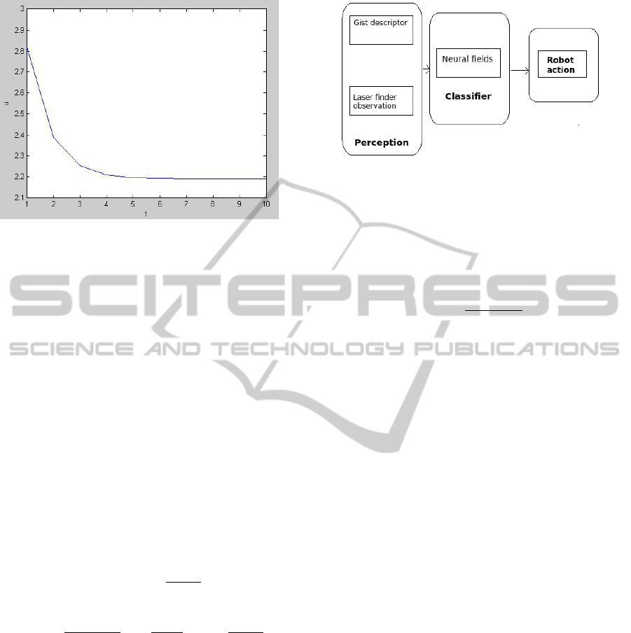
Figure 8: Activity of the neural field u(φ,t).
The state u(φ,t) depends on the stimuli S which
we will compute using a fusion scheme of GIST vi-
sual descriptor and Laser data. The computed signal
will allow us to determine the best action.
5.2.1 Laser Range Stimulus
We extract range and bearing information from the
Laser range sensors which are stimuli for the dynamic
neural field. These sensors give perceptions when
the robot is facing an obstacle, for example a hu-
man that moves randomly in an indoor environment.
Let’s consider the observation function h(X), where
X = (x,y, θ):
Z
t
= [r
k
t
, phi
k
t
]
T
The model of observation is given with:
Z
t
= h
t
(X
t
) = [
((delta))
arctan(
delta(2)
delta(1)
) − θ
t
]
S = C
0
∗ (
1
1 ∗ π
2
∗ σ
2
exp(
−r
2
2 ∗ σ
2
) ∗ exp(
−phi
2
2 ∗ σ
2
)
Where C
0
is the amplitude of the stimulus and σ is the
range of inhibition of the stimuli
5.2.2 Visual Stimulus
We consider the GIST vector as visual stimulus. It
quantifies the visual cue of an image which is very im-
portant when the robot navigates in an indoor environ-
ment because the objects may have different appear-
ances. Besides of that, the obstacles may be whatever
which sustain the choice of global features as stimuli.
We note that don’t use local features in spite of their
high distinctiveness because their calculation is time
consuming.
Figure 9: The scheme of our method of obstacle avoidance.
Lets have the GIST descriptor:
D = gist
i
/i = 1..N
gist
i
represents the i
th
component of the GIST de-
scriptor for an acuired image.
S
v
i
= exp(
g
2
i
2 ∗ sigma
2
)
Thus the equation of the GIST visual stimuli is given
with:
S
v
= (S
1
,S
2
,S
3
,...,S
N
)
N represents the dimension of the GIST descriptor.
6 OBSTACLE AVOIDANCE WITH
NEURAL FIELDS
The robot moves in a square environment using the
motion model p(x
t+1
/x
t
,u) affected with Gaussian
white noise (x
t+1
and x
t
are the robots positions at
time t+1 and t respectively, u is the odometry dis-
placement. When the robot is moving between two
estimated positions, we put an obstacle in the sur-
rounding of the robot. We change the action on the
robot if the distance separating the robot from the ob-
stacle is less that 0.7 meters.
Then we compute the stimuli used in the neural
field by computing the sum of the laser range finder
observation and the extracted visual GIST feature.
This computed observation is based on the calculus
of the distance and the directions of the laser sensor
and the global visual descriptor. This observation is
novel because it fuses two sensors: Laser range finder
and the camera. Therefore we compute the solution
of the Dynamic Neural Field given by the equa. 1.
We mentionne that this method is based on the learn-
ing decision paradigm. That’s why we start with the
contruction of 4 classes of the stimuli where each one
is associated to one of these actions (move right, left,
forward, backward). The fusion of the camera and the
AMulti-sensoryStimuliComputationMethodforComplexRobotBehaviorGeneration
143
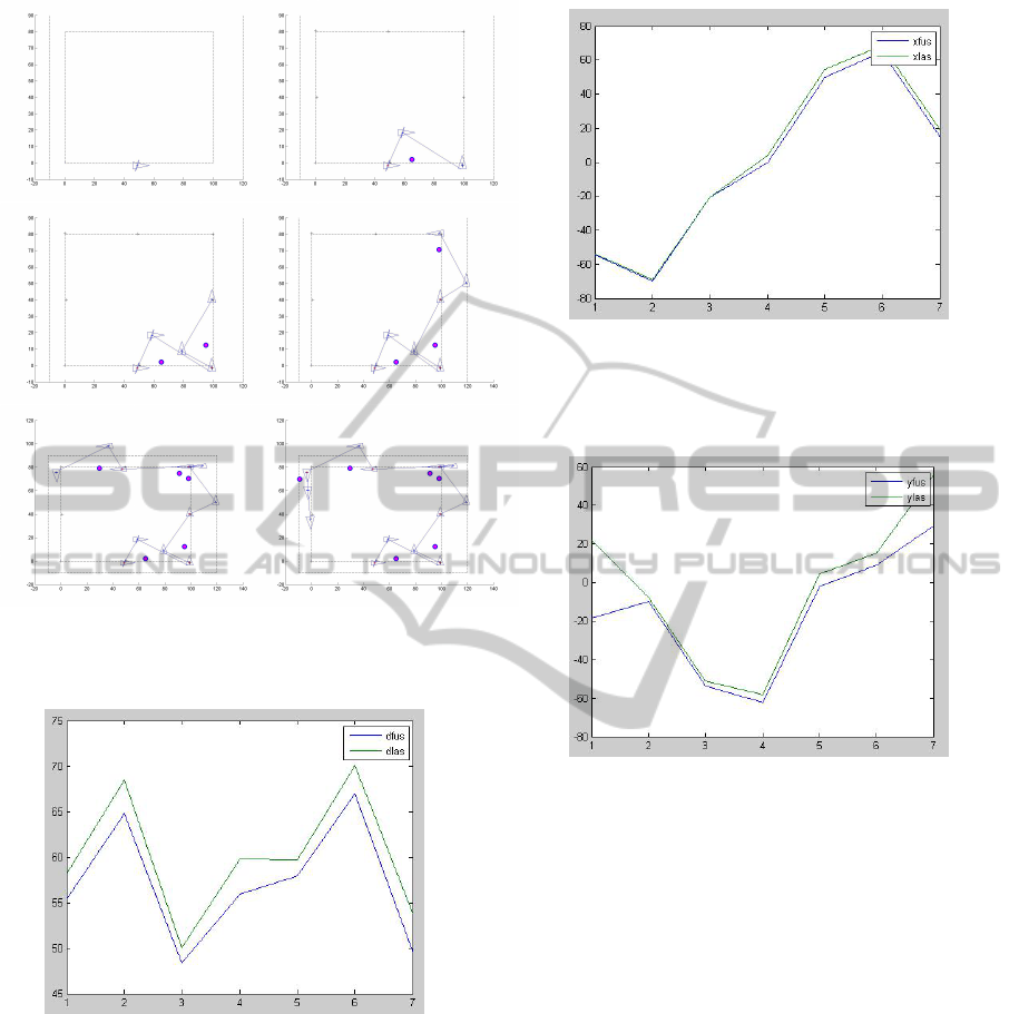
Figure 10: The robot motion with obstacle avoidance and
EKF, elementary behaviour of the robot is given with out-
puts of neural fields stimulated with laser range data.
Figure 11: Standard deviation of the error between the posi-
tions generated with neural field and the ground truth ( blue
for the fusion of multi sensory data and green for the laser
only data).
laser sensor data improve the accuracy of the robot lo-
calization. We show from the figures 11 12 13 that
the curve related to fusion is always lower that the one
of laser only.
7 CONCLUSION
We enhanced the accuracy of the robot navigation by
Figure 12: Standard deviation of the error on x coordinates
between the positions generated with neural field and the
ground truth ( blue for the fusion of multi sensory data and
green for the laser only data).
Figure 13: Standard deviation of the error on y coordinates
between the positions generated with neural field and the
ground truth ( blue for the fusion of multi sensory data and
green for the laser only data).
using two types of sensors, Camera and Laser range
finder, instead of only one. The neural field is good
because it is inspired from biological processes, so
the algorithm are better. We use GIST descriptor in-
stead of local feature points to increase the run time of
our program. Our method could be implemented on
mobile robots in dynamic environments to avoid ob-
stacles. The metrical navigation is more accurate than
the topological navigation, that is why we have used
it, through the application of the Extended Kalman
Filter to update the position when the robot avoids the
obstacle. We aim at the future to use neural field in
robot localization and mapping with the application
of topological mapping. We will focus on the im-
provement of the attractors dynamic that use neural
fields to move the robot with less error on the odome-
try displacements.
ICINCO2015-12thInternationalConferenceonInformaticsinControl,AutomationandRobotics
144

REFERENCES
Amari, S. (1977). Dynamics of pattern formation in lateral-
inhibition type neural fields. In Biological cybernet-
ics.
C. Crick, B. (2010). Controlling a robot with intention de-
rived from motion. In Topics in Cognitive Science,
pages 114–126.
Maja, M. (1992). Integration of representation into goal-
driven behavior-based robots. IEEE Transactions on
Robotics and Automation, 13:304 to 312.
M. Milford and G. Wyeth (2010). Persistent navigation and
mapping using a biologically inspired SLAM system.
Int. J. Robotics Research, 29(9):1131–1153.
Oliva, A. and A. Torralba (2001). Modeling the shape of
the scene: a holistic representation of the spatial en-
velope. International Journal of Computer Vision,
42:145–175.
P. Cisek (2006). Integrated neural processes for defining po-
tential actions and deciding between them: A compu-
tational model. In The Journal of Neuroscience, pages
9761–9770.
Yan, W., C.Weber and S. Wermter (2012). A neural ap-
proach for robot navigation based on cognitive map
learning. In Proc. of IJCNN.
Y. Raoui, E. H. Bouyakhf and M. Devy (2010). Image in-
dexing for object recognition and content based image
retrieval systems. International Journal of Research
and Reviews in Computer Sciences.
Y. Raoui, E. H. Bouyakhf and M. Devy (2011). Mobile
robot localization scheme based on fusion of rfid and
visual landmarks. In ICINCO.
Y. Sandamirskaya, M. Richter and G. Sch
¨
oner (2011). A
neural-dynamic architecture for behavioral organiza-
tion of an embodied agent. International Conference
on Development and Learning ICDL.
AMulti-sensoryStimuliComputationMethodforComplexRobotBehaviorGeneration
145
