Objective Assessment of Asthenia using Energy and Low-to-High

Spectral Ratio

Farideh Jalalinajafabadi

, Chaitaniya Gadepalli

, Mohsen Ghasempour

, Frances Ascott

Mikel Luj

, Jarrod Homer

and Barry Cheetham

School of Computer Science, University of Manchester, Oxford Road, Manchester, U.K.

Department of Otolaryngology, Manchester Royal Inﬁrmary,

Central Manchester University Hospitals Foundation Trust, Manchester, U.K.

Keywords:

GRBAS, Asthenia, MLR, KNNR.

Abstract:

Vocal cord vibration is the source of voiced phonemes. Voice quality depends on the nature of this vibration.

Vocal cords can be damaged by infection, neck or chest injury, tumours and more serious diseases such as

laryngeal cancer. This kind of physical harm can cause loss of voice quality. Voice quality assessment is

required from Speech and Language Therapists (SLTs). SLTs use a well-known subjective assessment ap-

proach which is called GRBAS. GRBAS is an acronym for a ﬁve dimensional scale of measurements of voice

properties which were originally recommended by the Japanese Society of Logopeadics and Phoniatrics and

the European Research for clinical and research use. The properties are ‘Grade’, ‘Roughness’, ‘Breathiness’,

‘Asthenia’ and ‘Strain’. The objective assessment of the G, R, B and S properties has been well researched and

can be carried out by commercial measurement equipment. However, the assessment of Asthenia has been less

extensively researched. This paper concerns the objective assessment of ‘Asthenia’ using features extracted

from 20 ms frames of sustained vowel /a/. We develop two regression prediction models to objectively esti-

mate Asthenia against speech and language therapists (SLTs) scores. These regression models are ‘K nearest

neighbor regression’ (KNNR) and ‘Multiple linear regression’(MLR). These new approaches for prediction

of Asthenia are based on different subsets of features, different sets of data and different prediction models

in comparison with previous approaches in the literature. The performance of the system has been evaluated

using Normalised Root Mean Square Error (NRMSE) for each of 20 trials, taking as a reference the average

score for each subject selected. The subsets of features that generate the lowest NRMSE are determined and

used to evaluate the two regression models. The objective system was compared with the scoring of each

individual SLT and was found to have a NRMSE, averaged over 20 trials, lower than two of them and only

slightly higher than the third.

1 INTRODUCTION

Perceptual and objective assessments of voice qual-

ity are widely used for voice disorder evaluation (Yu

et al., 2006; Wuyts et al., 2000; Jalalinajafabadi et al.,

2013). A single measurement cannot quantify all the

properties of an impaired voice that may be of inter-

est to clinicians. The ﬁve dimensional GRBAS scale

has the advantage of being widely understood and rec-

ommended by many professional bodies. The GR-

BAS scale is a 5-dimensional measurement of voice

quality where the dimensions are: ‘Grade’, ‘Rough-

ness’, ‘Breathiness’, ‘Asthenia’ and ‘Strain’(Hirano,

1981). ‘Grade’ represents overall degree of hoarse-

ness or voice abnormality.‘Roughness’ is irregular

ﬂuctuation in amplitude and fundamental frequency

of voicing source, ‘Breathiness’ arises from non-

periodic sound and an auditive impression of turbu-

lent air leakage through an insufﬁcient glottis closure.

‘Asthenia’ is weakness or lack of energy in the voice

and ‘Strain’ is difﬁculty in initiating and maintaining

voiced speech.

Each dimension is traditionally scored by Speech

and Language Therapists (SLTs) on a scale between

0 and 3; 0 for normal, 1 for mild impairment, 2 for

moderate impairment and 3 for severe impairment

(Hirano, 1981). Subjectivity and reliance on highly

trained personnel are signiﬁcant limitations of tradi-

tional ways of measuring GRBAS parameters. The

objective assessment of G, R, B and S properties has

Jalalinajafabadi F., Gadepalli C., Ghasempour M., Ascott F., Luján M., Homer J. and Cheetham B..

Objective Assessment of Asthenia using Energy and Low-to-High Spectral Ratio.

DOI: 10.5220/0005545000760083

In Proceedings of the 12th International Conference on Signal Processing and Multimedia Applications (SIGMAP-2015), pages 76-83

ISBN: 978-989-758-118-2

 2015 SCITEPRESS (Science and Technology Publications, Lda.)

been well researched and commercial equipment ex-

ists that is capable of doing this (Awan and Roy, 2006;

KayPENTAX, 2008). However, the assessment of

Asthenia has been less extensively researched. It is

one of the most difﬁcult components to score and

there is often more discrepancy between SLTs in As-

thenia scoring, than for the other dimensions. This

research is concerned with the objective assessment

of Asthenia (Hirano, 1981).

Patients with Asthenia might be referred to hospi-

tal for treatment. The weakness can caused by a low

intensity of the glottal source sound and is generally

associated with a lack of higher frequency harmonics

(Hirano, 1981). Figure 1 illustrates the methodology

of the approach. To assess a recorded voice signal

for Asthenia, it will be fed into a digital signal pro-

cessing system for extracting voice features such as

energy, pitch frequency variation, harmonic to noise

ratio and others. This followed by a mapping tech-

nique based on machine learning. The voice features

which reﬂect the lack of energy and higher frequency

harmonics will be extracted from the voice and used

as features by the mapping techniques.

Figure 1: Methodology of the Approach.

2 DATA COLLECTION AND

ASTHENIA SCORING

Voice data has been collected from a random selection

of 46 patients and 56 controls. Only participants that

can read English ﬂuently were included in this study.

All participants were adults between 18 and 70 years

of age, and they were in different stages of their treat-

ment. Information about the participants was stored in

secure ﬁles. The sustained acoustic signals were cap-

tured by a high quality Shure SM48 microphone that

was held a constant distance of 20 cm from the lips

and digitized using the KayPentax 4500 CSL Com-

puterized Speech Laboratory (KayPENTAX, 2008).

Each recording consists of two sustained vowels /a/

and /i/ lasting about 10 seconds, a set of six standard

sentences as speciﬁed by CAPE-V (Consensus for au-

ditory perception and evaluation) (Kempster et al.,

2009) and about 15 seconds of free unscripted speech.

To assess the voice quality of each participant sub-

jectively according to the GRBAS scale, the voice

samples were scored by three experienced SLTs using

Sennheiser HD205 head-phones. The samples were

played out in random order with 21 randomly cho-

sen samples repeated as a test for consistency. To

facilitate the scoring process, we developed a ‘GR-

BAS Presentation and Scoring Package’ (GPSP) for

collecting GRBAS scores. The graphical user inter-

face presented by this package is shown in Figure 2.

The software is designed to play out in random order,

with appropriate repetition, the voice samples from a

database of recordings. It enables scores to be entered

by the SLT and stored in the data-base as an excel

spread-sheet easily. The SLTs are given the option of

listening to any samples again, and the software can

be paused at any point, without loss of data. The user

may therefore take breaks to prevent tiredness which

may affect the scoring. The scoring of the 102 voice

samples referred to in this paper was completed by

each SLT in two sessions.

Both Pearson correlation and the Cohen’s Kappa

coefﬁcient were used to measure the level of agree-

ment in scoring Asthenia between each pair of SLTs

(Sheskin, 2003; Cohen, 1968). Equation (1) deﬁnes

the Pearson correlation (Sheskin, 2003) between the

two dimensions of a sample {(x

)} containing n

pairs of random variables (x

, y

) ; ¯x and ¯y are the

sample means of {x

} and {y

} respectively.

r =

∑

i=1

− ¯x)(y

− ¯y)

∑

i=1

− ¯x)

∑

i=1

− ¯y)

(1)

The Cohen Kappa coefﬁcient is deﬁned by Equa-

tion (2) where p

is the proportion (between 0 and 1)

of subjects for which the two SLTs agree on the scor-

ing, and p

is the probability of agreement ‘by chance’

when there is assumed to be no correlation between

the scoring by each SLT (Streiner, 1995; Viera et al.,

2005).

k =

− p

1 − p

(2)

Kappa is widely used for comparing raters or

scorers, and reﬂects any consistent bias in the aver-

age scores for each scorer (Viera et al., 2005) which

would be disregarded by Pearson’s correlation. A

value less than zero indicates no agreement. Values

in the range 0 to 0.2, 0.2 to 0.4, 0.4 to 0.6, 0.6 to 0.8

and 0.8 to 1 indicate slight, fair, moderate, substan-

tial and almost perfect agreement respectively (Viera

et al., 2005)

Weighted Kappa is often more appropriate when

there are more than two possible scores with a sense

of distance between the scores (Cohen, 1968). With

possible scores 0, 1, 2, 3, Kappa only considers

agreement or disagreement between scores, whereas

ObjectiveAssessmentofAstheniausingEnergyandLow-to-HighSpectralRatio

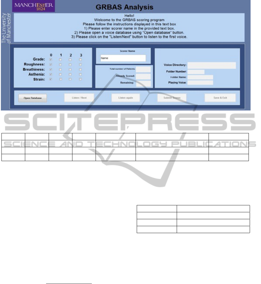
Figure 2: Screen shot of the GPSP.

Table 1: Kappa and Weighted Kappa (k

SLTs p

Kappa Agreement Weighted Kappa (k

) Agreement

1 & 2 0.64 0.48 0.316 Fair 0.311 Fair

2 & 3 0.63 0.50 0.327 Fair 0.317 Fair

1 & 3 0.68 0.38 0.483 Moderate 0.603 Moderate

weighted Kappa takes into account the degree of dis-

agreement. In this application, discrepancy between

scores 0 and 2, for example, is more serious than the

difference between 0 and 1 or between 1 and 2, and

weighted Kappa takes this into account. With lin-

early weighted Kappa (k

), the disagreement between

0 and 2 may be weighted twice that between 0 and 1,

1 and 2, or 2 and 3. The discrepancy between 0 and

3 may be weighted three times that between 0 and 1.

Equation (3) is a formula for linearly weighted Kappa

), where p

oij

is the proportion of subjects that are

scored i by scorer A and j by scorer B; p

eij

is the prob-

ability of scorer A scoring i while scorer B scores j,

for the observed distribution of scores by each scorer,

but with no correlation between scorers.

kw = 1 −

∑

i=0

∑

j=0

|i − j|p

oij

∑

i=0

∑

j=0

|i − j|p

eij

(3)

As results in Table 1 show, there is only fair

agreement between scorer 2 and scorers 3 and 1;

and better agreement between scorers 1 and 3. The

measured agreement between scorer 1 and scorer 3

changes signiﬁcantly when Kappa is replaced by lin-

early weighted Kappa. To make the Asthenia scores

more reliable, we can take some form of mean of the

three scores. We used the arithmetic mean or average.

If the means for all scorers are the same, Pearson

correlation is a good indicator of absolute agreement.

If the means are not the same, it can be misleading

if incorrectly interpreted. Table 2 shows the mean of

Asthenia scores for each SLT.

Table 2: Mean of Asthenia Scores.

SLT Mean of Asthenia Scores

SLT 1 0.63

SLT 2 0.30

SLT 3 0.76

3 ASTHENIA PREDICTION

3.1 Feature Extraction

The beginning and end of each sustained vowel were

trimmed to remove silence. Each sustained vowel was

divided into a series of non-overlapping 22.676 ms

(1000 sample) frames sampled at 44.1 kHz. For each

frame, the energy was computed. The mean energy

per frame (MEPF), the ratio of minimum to maximum

energy per frame energy (RMMEPF) were computed.

Also the standard deviation of the frame-by-frame en-

ergy (STD EPF) was calculated. The MEPF of each

vowel was normalized by dividing by the average of

the MEPF values obtained for all ‘normal’ voices out

of the 102 examples.

SIGMAP2015-InternationalConferenceonSignalProcessingandMultimediaApplications

To extract the ‘low-to-high spectral (L/H) ratio’,

each analysis frame was decimated by factor of 5,

‘zero-padded’, Hamming windowed and applied to a

400 point DFT. The spectral energy below and above

a cut-off frequency of 1.5 kHz was computed for each

frame and hence a low to high spectral ratio (L/H)

was obtained for each frame. This was averaged for

the whole recording to obtain a mean value of L/H

(ML/H). Other features such as the ratio of the max-

imum to minimum value of L/H (RMML/H) and the

standard deviation of L/H (STD L/H) were computed

for each vowel. The cut-off frequency 1.5 kHz was

selected due to most voiced speech energy occurring

below twice this frequency (i.e. about 3kHz). Six fea-

tures were created for predicting an Asthenia score for

each participant. Table 3 represents the six extracted

voice features.

Table 3: Deﬁnition of six extracted voice features.

Label Feature Deﬁnition

F1 MEPF Mean Energy Per Frame

F2 RMMEPF

Ratio of Minimum to

Maximum Energy Per

Frame

F3 STD EPF

Standard Deviation of

Energy Per Frame

F4 ML/H

Mean of Low to High

Spectral Ratio

F5 RMML/H

Ratio of Minimum to

Maximum Low to High

Spectral Ratio

F6 STD L/H

Standard Deviation of Low

to High Spectral Ratio

3.2 Feature Selection Method

Feature selection methods can determine a subset of

the available features that will give the best accuracy

in predicting Asthenia. They can be used to identify

and remove unnecessary, irrelevant and redundant at-

tributes from data that do not contribute to the accu-

racy of a predictive model or even increase the error

of the prediction. Wrapper methods were used as the

feature selection method in predicting Asthenia (Yuan

et al., 1999; Kohavi and John, 1997; Langley et al.,

1994).

Wrapper methods train a new model for each pos-

sible subset of features. These methods assess subsets

of variables according to their usefulness to a given

predictor. The method conducts a search for a good

subset using the learning algorithm itself as part of

the evaluation function. ‘Wrapper’ methods are com-

putationally intensive, but usually provide the best

performing subset of features (Guyon and Elisseeff,

2003). Greedy Forward Search, Exhaustive Search

are two examples of wrapper methods (Langley et al.,

1994).

In this research, ‘Exhaustive Search’ was used.

This method is looking at every possible combination

of features to ﬁnd which one gives the best result. It

is only possible to do this with a small number of fea-

tures and so some simpliﬁcation of this problem must

be done. A straightforward wrapper method was de-

veloped in MATLAB to test all possible subsets of

features. With n features there are 2

−1 possible sub-

sets. Therefore, with 6 features, there are 63 different

feature subsets.

3.3 Prediction Models

Linear regression (MLR) and K-nearest-neighbor- re-

gression (KNNR) (Berry and Feldman, 1985; Jiang-

sheng, 2002) were used and compared for the objec-

tive prediction of Asthenia. The average of three SLTs

scores were considered as the true value of the Asthe-

nia scores. Regression was used rather than classiﬁca-

tion in order to take account of the magnitudes of the

differences between the scores, which are signiﬁcant

with GRBAS scoring.

3.3.1 Feature Scaling

To improve the performance of the prediction mod-

els, features were scaled to make the mean of each

feature equal to zero and the standard deviation equal

to 1. Refer to F

as feature j for participant i. Refer

to feature F

before scaling as F

ij(non-scaled)

and after

scaling as F

ij(scaled)

. Let

and σ

denote the sample-

mean and the sample-standard-deviation respectively

of non-scaled feature j over all n participants. The

scaled version of each feature F

for participant i is

then:

ij(scaled)

ij(non-scaled)

−

(4)

3.3.2 MLR Performance in Asthenia Prediction

To test the capability of the MLR method for Asthe-

nia prediction, and to ﬁnd out which subset of features

it is the best to use, twenty ‘trials’ were carried out

whereby random selections of 80 recording examples

were used for a cross-validation (training set and vali-

dation set) procedure and the remaining 22 recordings

were used for the testing. The experiment was applied

to the database of 102 recordings. In each trial, 63 dif-

ferent subsets of features selected from the 6 features,

were taken. For each subset, the validation error was

calculated using 10 fold cross validation. The subset

ObjectiveAssessmentofAstheniausingEnergyandLow-to-HighSpectralRatio

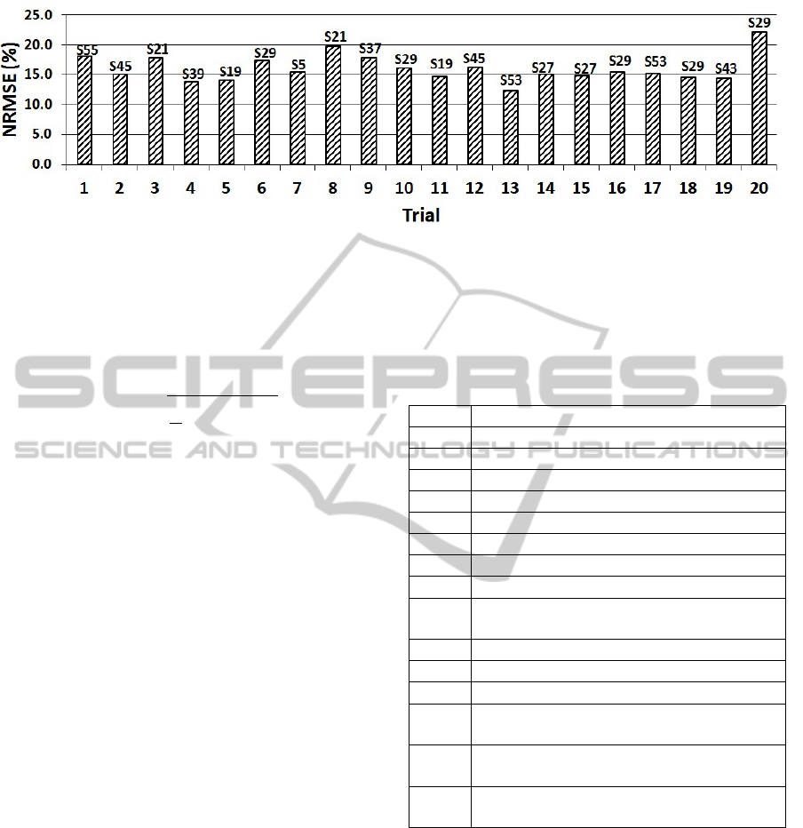
Figure 3: NRMSE for the best subset in each trial (MLR).

which gives the lowest RMSE over the validation set

was used for a training using 80 examples and testing

on 22 examples and the generalisation error was com-

puted. The RMSE between the predicted (

Y ) and the

observed value (Y) for 22 (N) recording examples is:

RMSE =

∑

i=1

(

−Y

)

(5)

Table 4 deﬁnes the subset of features that are re-

ferred to in Figure 3. Figure 3 depicts the NRMSE as

generalisation error on 22 examples for the best sub-

set of feature found in each trial. S21 was ﬂagged

as the best subset several times (i.e. ﬁve times) with

NRMSE error 17.81%, 17.87%, 14.80%, 15.22% and

22.13% respectively over 20 trials, where NRMSE is:

NRMSE = RMSE/(Asthenia

max

−Asthenia

min

)∗100

(6)

3.3.3 Best Feature Subset Selection and Optimal

K for KNNR

With KNNR, the RMSE of the regression will be af-

fected by the feature subset and value of K, which is

the number of nearest neighbors chosen. We used 10

fold cross-validation (Kohavi et al., 1995) on 80 ran-

dom examples to determine the RMSE on validation

sets for each subset for K in range of 1 to 10. In each

trial, a grid search (Bergstra and Bengio, 2012) was

used to ﬁnd out the best feature subset and optimal K

with the lowest RMSE amongst 63 different subsets.

To measure the performance of the KNNR model on

unseen examples by generalisation error, the best sub-

set with the optimal K was used on 80 random train-

ing set and 22 random testing examples . This ex-

periment was carried out for 20 different trials and

the generalisation error was computed as NRMSE in

each trial. Figure 5 shows the NRMSE for the best

subset in each trial. Figure 4 illustrates the optimal

K for the best subset in each trial. S15 was ﬂagged

several times (i.e. ﬁve times) as the best subsets over

20 trials with 18.12%, 17.95%, 17.28%, 14.91% and

16.90% NRMSE respectively.

Table 4: Deﬁnition of feature subsets referred to in Figures

3,4 and 5.

Subset Deﬁnition

S3 STD EPF, RMMEPF

S7 MEPF, STD EPF, RMMEPF

S11 RMML/H, STD EPF, RMMEPF

S13 RMML/H, MEPF, RMMEPF

S15 RMML/H, MEPF, STD EPF, RMMEPF

S19 STD L/H, STD EPF, RMMEPF

S21 STD L/H, MEPF, RMMEPF

S23 STD L/H, MEPF, STD EPF , RMMEPF

S27

STD L/H ,RMML/H, STD EPF,

RMMEPF

S35 ML/H, STD EPF, RMMEPF

S37 ML/H, EPF, RMMEPF

S39 ML/H, MEPF, STD EPF, RMMEPF

S43

ML/H, RMMML/H, STD EPF,

RMMEPF

S47

ML/H, RMML/H, MEPF, STD EPF,

RMMEPF

S61

ML/H, STD L/H, RMML/H, MEPF,

RMMEPF

4 COMPARISON BETWEEN MLR

AND KNNR

The performance of the MLR and KNN techniques

were compared for predicting Asthenia objectively.

The standard deviation of the error may be investi-

gated to estimate the stability of the models. For

MLR, the mean and standard deviation of error for the

best subsets over 20 trials are about 16.06% and 2.25

respectively with 95% conﬁdence limits at 15.1% and

17% over 20 trials. KNN makes this mean and stan-

SIGMAP2015-InternationalConferenceonSignalProcessingandMultimediaApplications

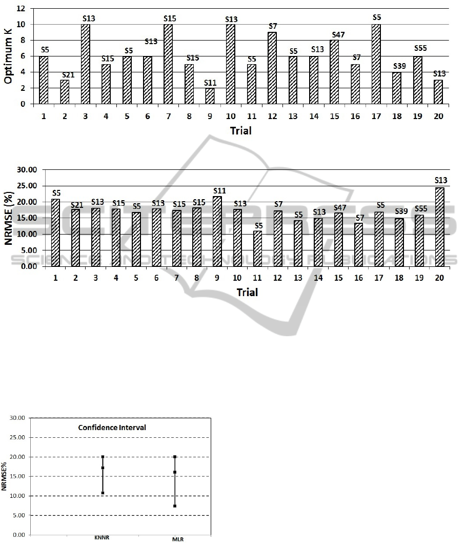
Figure 4: Best K for the best selected feature subset in each trial.

Figure 5: NRMSE for the best selected feature subset in each trial (KNNR).

dard deviation of the error 17.20% and 2.92 respec-

tively with 95% conﬁdence limits at 15.9% and 18.5%

over 20 trials. Figure 6 displays no statistically sig-

niﬁcant difference between the models because of the

overlap in the conﬁdence interval of both models but

KNNR has lower standard deviation in error and the

error is more closely clustered around mean.

Figure 6: Conﬁdence Interval.

5 OBJECTIVE SYSTEM VS

PERCEPTUAL SCORING

The objective system over 20 trials, using the best

subset of features, has an average of NRMSE around

16.06% and 17.20% by MLR and KNN respectively.

For each of these prediction models NRMSE was

computed over 22 examples. To evaluate the objec-

tive system and each scorer against the average of

three SLTs, the NRMSE was computed for the objec-

tive system and each individual SLTs who are rated

the same number of patients (22 examples) in the 20

trials. Figure 7 shows the NRMSE between the three

SLTs, the KNNR model and the MLR where average

of the 3 scorers taken as the reference. On average,

for both objective prediction models, the NRMSE

is lower than that obtained for SLT2 and SLT1 and

higher than that obtained for SLT3.

6 RELATED WORK

Objective assessment of voice has been studied ex-

tensively (Villa-Canas et al., 2013; Bhuta et al., 2004;

Yu et al., 2006; Wuyts et al., 2000). Considering the

GRBAS dimensions, Asthenia has not been as widely

covered as the others. A recent paper (Villa-Canas

et al., 2013) uses a K Nearest Neighbor classiﬁer to

predict all parameters using spectral energy measure-

ments, cepstral coefﬁcients, a glottal-to-noise excita-

tion ratio and other parameters. The objective scores

ObjectiveAssessmentofAstheniausingEnergyandLow-to-HighSpectralRatio

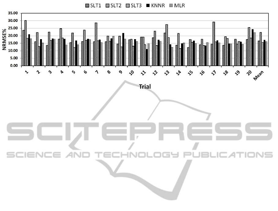
Figure 7: Comparison between NRMSE for three SLTs and objective system (KNNR and MLR).

were compared with perceptual evaluations by a sin-

gle expert at the University Poletecnica of Madrid.

Good correspondence were obtained, the best efﬁ-

ciency, 89.3%, being obtained for Asthenia (Villa-

Canas et al., 2013) . Our work uses a different data-

base, three experienced SLT scorers and a different

feature set. Also we use regression models rather than

classiﬁcation, and compare two regression models.

Regression is sensitive to the degree of disagreement

between scores where classiﬁcation is concerned only

with agreement or disagreement.

7 CONCLUSIONS AND FUTURE

WORK

The proposed schemes are intended to be used for

the objective assessment of Asthenia according to the

GRBAS scale. The average of the three Asthenia

scores obtained by SLTs 1, 2 and 3 was assumed to be

the best possible estimate of the true Asthenia score

for each subject in this experiment.

The objective measurement of Asthenia was ob-

tained using multiple linear regression and K-nearest

neighbor regression by combinations of energy and

low to high spectral measurement for sustained vowel.

The use of low to high spectral ratio and energy per-

mits estimation of Asthenia without the limitations as-

sociated with traditional time-based dysphonia mea-

sures such as jitter and shimmer.

For both prediction models the best feature subset

was selected based on the lowest validation error in

each trial. Moreover, MEPF, RMMEPF, RMML/H

and the STD L/H features were found to be the

strongest contributors.

The average of generalisation error (NRMSE)

over 20 trials was measured for KNNR and MLR

which is less than 17.20% in both models.

It is now necessary to apply the approach in this

paper to the data-base used by Villa et al. (Villa-Canas

et al., 2013) to compare the values of Asthenia ob-

tained. Different methods can be proposed for the de-

cision about the true Asthenia scores which may give

different results from averaging in prediction. The

use of connected speech as well as sustained vowels

should also be introduced since this is used by SLTs.

Future studies with larger samples of voice disorder

types and severities are then needed.

ACKNOWLEDGEMENTS

This work is partly supported by EPSRC grant

AnyScale Apps EP/L000725/1. Mikel Luj

an is

funded by a Royal Society University Research Fel-

lowship.

REFERENCES

Awan, S. N. and Roy, N. (2006). Toward the development

of an objective index of dysphonia severity: a four-

factor acoustic model. Clinical linguistics & phonet-

ics, 20(1):35–49.

Bergstra, J. and Bengio, Y. (2012). Random search for

hyper-parameter optimization. The Journal of Ma-

chine Learning Research, 13(1):281–305.

Berry, W. D. and Feldman, S. (1985). Multiple regression

in practice. Number 50. Sage.

Bhuta, T., Patrick, L., and Garnett, J. D. (2004). Percep-

tual evaluation of voice quality and its correlation with

acoustic measurements. Journal of Voice, 18(3):299–

304.

Cohen, J. (1968). Weighted kappa: Nominal scale agree-

ment provision for scaled disagreement or partial

credit. Psychological bulletin, 70(4):213.

Guyon, I. and Elisseeff, A. (2003). An introduction to vari-

SIGMAP2015-InternationalConferenceonSignalProcessingandMultimediaApplications

able and feature selection. The Journal of Machine

Learning Research, 3:1157–1182.

Hirano, M. (1981). Clinical examination of voice, volume 5.

Springer New York.

Jalalinajafabadi, F., Gadepalli, C., Ascott, F., Homer, J.,

Luj

an, M., and Cheetham, B. (2013). Perceptual eval-

uation of voice quality and its correlation with acous-

tic measurement. In Modelling Symposium (EMS),

2013 European, pages 283–286. IEEE.

Jiangsheng, Y. (2002). Method of k-nearest neighbors. In-

stitute of Computational Linguistics, Peking Univer-

sity, China, 100871.

KayPENTAX (2008). A Division of PENTAX medical

Company. http://www.kaypentax.com. [Accessed 19-

March-2015].

Kempster, G. B., Gerratt, B. R., Abbott, K. V., Barkmeier-

Kraemer, J., and Hillman, R. E. (2009). Consensus

auditory-perceptual evaluation of voice: development

of a standardized clinical protocol. American Journal

of Speech-Language Pathology, 18(2):124–132.

Kohavi, R. et al. (1995). A study of cross-validation and

bootstrap for accuracy estimation and model selection.

In IJCAI, volume 14, pages 1137–1145.

Kohavi, R. and John, G. H. (1997). Wrappers for feature

subset selection. Artiﬁcial intelligence, 97(1):273–

324.

Langley, P. et al. (1994). Selection of relevant features

in machine learning. Defense Technical Information

Center.

Sheskin, D. J. (2003). Handbook of parametric and non-

parametric statistical procedures. crc Press.

Streiner, D. L. (1995). Learning how to differ: agreement

and reliability statistics in psychiatry. The Canadian

Journal of Psychiatry/La Revue canadienne de psychi-

atrie.

Viera, A. J., Garrett, J. M., et al. (2005). Understanding in-

terobserver agreement: the kappa statistic. Fam Med,

37(5):360–363.

Villa-Canas, T., Orozco-Arroyave, J., Arias-Londono, J.,

Vargas-Bonilla, J., and Godino-Llorente, J. (2013).

Automatic assessment of voice signals according to

the grbas scale using modulation spectra, mel fre-

quency cepstral coefﬁcients and noise parameters.

In Image, Signal Processing, and Artiﬁcial Vision

(STSIVA), 2013 XVIII Symposium of, pages 1–5.

IEEE.

Wuyts, F. L., De Bodt, M. S., Molenberghs, G., Remacle,

M., Heylen, L., Millet, B., Van Lierde, K., Raes,

J., and Van de Heyning, P. H. (2000). The dyspho-

nia severity indexan objective measure of vocal qual-

ity based on a multiparameter approach. Journal of

Speech, Language, and Hearing Research, 43(3):796–

809.

Yu, P., Garrel, R., Nicollas, R., Ouaknine, M., and Gio-

vanni, A. (2006). Objective voice analysis in dyspho-

nic patients: new data including nonlinear measure-

ments. Folia Phoniatrica et Logopaedica, 59(1):20–

30.

Yuan, H., Tseng, S.-S., Gangshan, W., and Fuyan, Z.

(1999). A two-phase feature selection method using

both ﬁlter and wrapper. In Systems, Man, and Cyber-

netics, 1999. IEEE SMC’99 Conference Proceedings.

1999 IEEE International Conference on, volume 2,

pages 132–136. IEEE.

ObjectiveAssessmentofAstheniausingEnergyandLow-to-HighSpectralRatio