Polarization Dependent Loss Emulator Built with Computer-driven

Polarization Controllers and Single Mode Fibre

Yangzi Liu, Peter Shepherd and Duncan Allsopp

Department of Electronic and Electrical Engineering, University of Bath, Bath, U.K.

Keywords:

Polarization Dependent Loss, Polarization Components Positioning.

Abstract:

In this paper, a polarization dependent loss emulator is designed with computer-driven polarization controllers

and single mode ﬁbre. It proves that PDL obeys Maxwellian distribution when it is expressed in decibels. By

positioning the polarization controllers at different places in the emulator link, it also proves that positions of

PDL components have a signiﬁcant effect on the statistics of PDL in a ﬁxed length communication system.

As the number of polarization components involved and the communication ﬁbre length remain as constants,

the longer the uninterrupted ﬁbre is, the smaller the PDL mean value is produced.

1 INTRODUCTION

Optical ﬁbre communication networks are playing an

important role in the area of high-speed, high-volume

and ultralong-distance data transmission. With the

growth in demand for greater data, greater bandwidth

has been applied, this has made polarization become

an effect which cannot be ignored in the system. For

example, polarization has been considered as a major

obstacle in the development of polarization-division-

multiplexing digital coherent transmission systems

when it is operating at more than 100Gb/s (Mori et al.,

2011). Polarization happens because of the asym-

metry of optical ﬁbre factors on the two orthogonal

axes, such as the asymmetry of dispersion parameters

which introduce polarization mode dispersion and the

asymmetry of loss parameters which introduce polar-

ization dependent loss. In the effect of polarization,

signals in the optical ﬁbre transmission systems will

be distorted by a bigger bit error rate, and a lower

signal-to-noise ratio.

As the optical pulse becomes narrower, polariza-

tion impairs transmission signals in two ways. Polar-

ization mode dispersion (PMD) can cause the signal

distortion due to the differential group delay (DGD)

on the two perpendicular axes in the ﬁbre, and polar-

ization dependent loss (PDL) can introduce additional

loss because of the difference of loss factor of the two

perpendicular axes in the ﬁbre. Moreover, PMD and

PDL always exist together in real optical transmission

systems, which generates combined effects. For ex-

ample, due to the loss of orthogonality between the

two principal states of polarization, PDL distorts the

statistics results of PMD away from the theoretical

distribution (Musara et al., 2013).

Even though PDL is limited to a relatively small

value in the latest produced ﬁbre (about 0.02dB/km

at 1550 nm), its time-dependent randomness makes it

a factor of reducing signal-to-noise ratio which can-

not be ignored (Lichtman, 1995), especially in those

old deployed ﬁbre communication systems. In order

to improve the performance of a long-distance opti-

cal transmission system, it is signiﬁcant to deploy a

proper number of polarization dependent ampliﬁers

in the proper positions. To achieve this target, a reli-

able PDL emulator is essential.

In this paper, a PDL emulator is built with

computer-driven polarization controllers and sections

of single mode ﬁbre. It is aimed to provide a continu-

ous statistical result which obeys the Maxwellian dis-

tribution, as concluded by previous researchers. An-

other goal of building this emulator is to ﬁnd out how

the PDL components work with communication ﬁ-

bres. To achieve this, the ﬁbre length of this emu-

lator is ﬁxed to a constant length (7×15 metres) and

two polarization controllers are used to provide ran-

dom states of polarization. One of the controllers is

constantly deployed between the laser source and the

ﬁrst link of ﬁbre and the other one is deployed at dif-

ferent places in the emulator in different cases. The

results are used to compare how the statistical results

are affected by the position changes of the second po-

larization controller.

Liu Y., Shepherd P. and Allsopp D..

Polarization Dependent Loss Emulator Built with Computer-driven Polarization Controllers and Single Mode Fibre.

DOI: 10.5220/0005563700420047

In Proceedings of the 6th International Conference on Optical Communication Systems (OPTICS-2015), pages 42-47

ISBN: 978-989-758-116-8

 2015 SCITEPRESS (Science and Technology Publications, Lda.)

2 POLARIZATION DEPENDENT

LOSS (PDL)

2.1 Deﬁnition

Polarization dependent loss is a measure of the peak-

to-peak difference in transmission of an optical com-

ponent or system with respect to all possible states of

polarization. It is deﬁned as the ratio of the maximum

and the minimum transmission of an optical device

with respect to all polarization states, as shown in Eq.

(1)

PDL

= 10 ×log(

Max

Min

) (1)

In Stokes space, a polarized light beam can

be written in the form of Stoke vector

S =

)

, where

= I

= I p cos 2ψ cos 2χ

= I p sin 2ψ cos 2χ

= I p sin 2χ

Here I p, 2ψ and 2χ are the spherical coordinates in

Stokes space, so the Stoke vector

S can present any

polarization state of the polarized light beam.

After passing through a device which changed the

state of polarization, the Stoke vector of this light

beam can be described as

out

= M

S where M is the

Muller Matrix used to describe the polarization device

M =













The output power of this light beam

out

= m

+ m

(2)

By the deﬁnition of Stokes vector, there is

= S

+ S

(3)

and P

out

can come to the extrema with the condition of

= k. Maximum or minimum values

are achieved respectively when k is positive or nega-

tive. Therefore, Eq. (1) can be rewritten as

PDL

= 10 ×log(

+ m

−

+ m

) (4)

2.2 The Statistical Theory

As polarization is a time-dependent element in trans-

mission systems, PDL plays its role as a random

attenuator. It generates irregularities in the power

evolution along the link and may cause a signiﬁcant

degradation in the optical signal-to-noise ratio. Previ-

ous research showed that for all the relevant range of

parameters the PDL of a communication system has

Maxwellian distribution when it is expressed in deci-

bels.

Even though the distribution of PMD obeys

Maxwellian distribution as well, the distribution of

PDL is independent of the system’s PMD (Mecozzi

and Shtaif, 2002). The dependence of the mean-

square PDL (in decibels) on system length is linear

in most cases, but it may become exponential in sys-

tems extending over transoceanic lengths.

The polarization dependent component of the

power gain of a generic optical element can be de-

scribed as 1 +

Γ ·

, where

is a unit Stokes vec-

tor corresponding to the polarization state of the inci-

dent optical ﬁeld and

Γ represents the vector of PDL.

Therefore, the highest and lowest gains are 1 ±Γ

with Γ = |

Γ| and the high gain is achieved when

is parallel to

Γ in Stokes space, and the lowest gain

is achieved when

is anti-parallel to

Γ. Based on

the deﬁnition of PDL, it can be described as PDL ≡

10log

[(1 + Γ)/(1 −Γ)]. In order to derive the PDL

distribution, the evolution equation of

Γ obtained by

Huttner (Huttner et al., 2000) is considered.

∂

∂z

β ×

Γ +

α −

Γ(

α ·

Γ). (5)

The vector

β(ω,z) is the local birefringence and α(z)

is the local vector of polarization dependent loss. ω

is the optical frequency and z is the position along the

ﬁbre link.

By considering the transmission system as con-

sisting of a large number of elements that contribute

to PDL in a statistically independent way, it can be

assumed that PDL vectors of the individual elements

are Gaussian vectors in Stokes space so that their ori-

entation is uniformly distributed. Therefore, the ﬁrst

term on the right hand side of Eq. (5) can be omit-

ted. It is arbitrary to assume that the local PDL vec-

tors have Gaussian distributed components. However,

it becomes irrelevant when the number of PDL ele-

ments in the system is large enough (Poole and Nagel,

1997). Now the PDL vector can be described as an

individual element by ηd

W , where d

W is an incre-

ment of a standard three-dimensional Brownian mo-

tion (Gardiner, 1985) and its most relevant property

is d

W ·d

W = dz. Therefore, the mean-square value

PolarizationDependentLossEmulatorBuiltwithComputer-drivenPolarizationControllersandSingleModeFibre

of the local PDL element is η

dz where η is a con-

stant. To simplify the notation, the position parame-

ter z can be normalized such that η

= 1. The nor-

malized z should be interpreted as the accumulated

sum of mean-square PDL values from the system in-

put (where z = 0) to any given point along the link.

With these assumptions, Eq. (5) can be rewritten in a

stochastic differential form

Γ = d

W −

Γ(d

W ·

Γ) −

Γ(2 −Γ

)dz (6)

where the last term is the byproduct of translating a

physical differential equation such as Eq. (5) into a

stochastic differential equation. With the relation be-

tween

Γ and ρ, the stochastic equation for ρ can be

written as

dρ =

γ/3

tanh(ρ/γ)

dz +

√

dW (7)

where ρ ≡20/ln(10) w 8.7 and the scalar dW is an in-

crement of a one-dimensional Brownian motion satis-

fying dW

= dz. A new vector process

ρ(z) in Stokes

space is introduced to obtain the distribution of ρ,

such as

ρ = [

ρ/γ

tanh(ρ/γ)

−1]

3ρ

dz + γd

W (8)

and it has the relation ρ = |

ρ|. It shows the stochastic

equation for

ρ ·

ρ is identical to Eq. (7). While

has no obvious physical interpretation, it is useful for

deriving the distribution of ρ, because Eq. (8) can

be approximated by performing a Taylor expansion

of the ﬁrst term on its right-hand side

ρ = [1 −

15γ

315γ

···]

ρdz + γd

W (9)

If the ﬁrst term in the square brackets in Eq. (9) is

considered, a linear equation is obtained , whose solu-

tion is a random vector with three independent Gaus-

sian components of zero mean and variance σ(z)

3γ

/2(e

2z/9

−1). Therefore, the distribution of ρ is

Maxwellian and it is given by

(ρ) =

4ρ

√

π[2σ

(z)]

3/2

exp[−

2σ

(z)

] (10)

The above approximation should be valid as long

as the second term in the expansion is signiﬁcantly

smaller than one (i.e., ρ

 15γ

), a condition that

is well satisﬁed for values of ρ  34 dB. The mean-

square value of the PDL is

hρ

i = 3σ(z)

9γ

2z/9

−1) (11)

and the mean PDL is given by hρi =

8hρ

i/(3π),

a relation that is deﬁned by the Maxwellian distri-

bution. Eq. (11) can be approximately written as

hρ

i w γ

z when 2z/9  1, where z is the accumu-

lated local mean-square PDL of the system.

Eq. (11) shows that the mean PDL exponentially

increases along the ﬁbre for long distance transmis-

sion but it can be seen as approximately linear when

the distance is small enough.

2.3 Effect in Long Distance

Transmission Systems

The PDL factor in modern built single mode ﬁbre is

about 0.02dB/km at the wavelength of 1550nm which

is relatively small (standard attenuation in the same

kind of single mode ﬁbre is about 0.2dB/km) and its

increase is approximately linear. However, the mean

value of PDL increases exponentially with distance

increasing in a ultralong-distance system, for exam-

ple, hundreds or thousands of kilometres. This can be

even worse in the old systems which were deployed

decades ago.

PDL will affect ultralong-distance systems in an-

other way. It can cause a signiﬁcant degradation in

the optical signal-to-noise ratio because it is randomly

changing with time. In order to compensate PDL,

polarization dependent ampliﬁers (ﬁbre-based Raman

ampliﬁers) are applied along the systems. In order

to achieve a better performance, the polarization de-

pendent ampliﬁers (PDA) are expected to have the

Maxwellian distribution related to the distribution of

PDL in the system. Therefore, it is signiﬁcant to un-

derstand the relationship between polarization com-

ponents and communication ﬁbres, not only the work-

ing parameters, but also the optimum positions of po-

larization components.

When the PDL is signiﬁcant, there is interaction

between PMD and PDL and that caused some com-

bined effects. In the presence of both PMD and

PDL, the two states of polarization are not orthogonal,

which leads to interferences producing anomalously

large pulse spreading (Gisin and Huttner, 1997).

3 EMULATOR DESIGN

The PDL emulator described in this paper is de-

signed with computer-drived polarization controllers

connected with sections of single mode ﬁbre. Polar-

ization controllers can provide random states of po-

larization in time to simulate and enhance the PDL

variation in the real situation, and they are connected

with single mode ﬁbre, which is used as the device

under test (DUT).

A stable laser source is used to provide continu-

ous lightwave at the wavelength of 1550 nm. A power

OPTICS2015-InternationalConferenceonOpticalCommunicationSystems

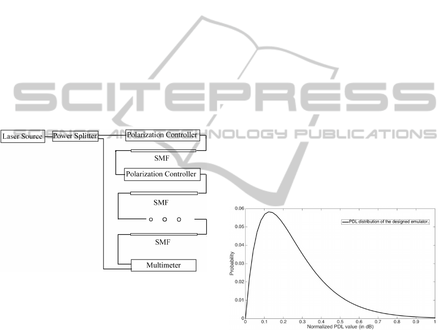
splitter is deployed between the laser source and the

system. 10% of the source power is sent to one chan-

nel of the multimeter as reference, and the other 90%

goes into the emulator.

The sections of single mode ﬁbre which are used

to connect each polarization controllers are 15 metres

long, as shown in Figure 1. All of the polarization

controllers are changing their paddle positions rapidly

and randomly to maximize the system randomization.

The system randomness is relative to the number

of polarization controllers applied. By changing this

it can be compared how PDL components in the trans-

mission system affect the statistical results of the out-

put PDL at the receiver. By changing the number of

sections of optical ﬁbre, it will give different results

corresponding to the different transmission distance.

Another variable in the emulator system is the posi-

tions of polarization controllers. By changing this, it

can be helpful to ﬁnd out the effect of PDL compo-

nent position changing and the relationship of PDL

component position and the transmission distance.

Figure 1: Emulator design.

By using the Stokes vector and Muller Matrix

which are discussed in Section 2.2, the emulator can

be described mathematically as

out

= F

...F

p+2

p+1

...F

S (12)

where M

and M

represent the polarization con-

trollers and F

,...F

represent the sections of sin-

gle mode ﬁbre. M

and M

generate random states

of polarization to optimum the measurement results.

By assuming the states of polarization do not change

within the relative short distance (15 metres), the

Muller Matrix of ﬁbre can be written as

= F

= ...F







exp(−αL) 0 0 0

0 1 0 0

0 0 1 0

0 0 0 1







(13)

where α is the loss parameter of the ﬁbre and L is the

length of ﬁbre. By combining the Muller Matrices

of coherent sections of ﬁbres, Eq. (12) can be also

written as

out

= F

n−t

S (14)

where







exp(−αpL) 0 0 0

0 1 0 0

0 0 1 0

0 0 0 1













exp(−α(n − p)L) 0 0 0

0 1 0 0

0 0 1 0

0 0 0 1







4 EXPERIMENTAL RESULTS

As described in the theoretical calculation, the statisti-

cal result of PDL obeys the Maxwellian distribution.

In order to check whether the statistical distribution

matches the theoretical calculation, the emulator runs

for 24 hours continuously to generate a statistical re-

sult, which is shown in Fig. 2. The probability curve

indicates that the result obeys Maxwellian distribu-

tion, which means the emulation results generated by

this emulator is reliable to be used to study polariza-

tion dependent loss in a laboratory environment.

Figure 2: The statistical result of the designed emulator

obeys Maxwellian distribution.

Based on Eq. (8), the mean-square value of the

PDL ρ

exponentially increases as the communica-

tion length increases. However, even if the commu-

nication distance is ﬁxed to a constant, the statistical

results in the system varies. By assuming the commu-

nication ﬁbre is in a constant of state of polarization,

the main factor which varies the statistical results is

the PDL components.

The PDL components statistically vary the results

in two ways. Their random patterns change as their

working environment changes in time. On the other

hand, the positions where the PDL components were

PolarizationDependentLossEmulatorBuiltwithComputer-drivenPolarizationControllersandSingleModeFibre

deployed in the systems can lead to different results

as the combination of PDL component and the ﬁ-

bre length is changed. In order to study the relation-

ship between the statistical results and the position of

PDL components, the emulator is set in seven differ-

ent cases (shown in Table 1). Polarization controller 1

is ﬁxed between the laser source and the ﬁrst section

of ﬁbre to provide an initial state of polarization and

polarization controller 2 is deployed in different posi-

tions in different cases. Fibre length of each section

is 15 metres.

Table 1: Case list of the different sets of emulator. PC1

and PC2 indicate polarization controller 1 and polarization

controller 2 respectively, SMF indicates single mode ﬁbre.

Case 1 PC 1−→ PC 2−→7 sections of SMF

Case 2 PC 1−→ 1 section of SMF−→PC 2−→6 sections of SMF

Case 3 PC 1−→ 2 sections of SMF−→PC 2−→5 sections of SMF

Case 4 PC 1−→ 3 sections of SMF−→PC 2−→4 sections of SMF

Case 5 PC 1−→ 4 sections of SMF−→PC 2−→3 sections of SMF

Case 6 PC 1−→ 5 sections of SMF−→PC 2−→2 sections of SMF

Case 7 PC 1−→ 6 sections of SMF−→PC 2−→1 section of SMF

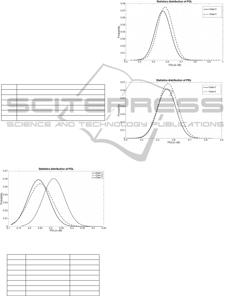
The emulator runs continuously for 24 hours as

one experimental period. Measurements were taken

multiple times in each case to achieve a better statis-

tical result. Figure 3, 4 and 5 show the distribution

curve of PDL in all of the cases and Table 2 shows

the mean value and variance of measured PDL in all

of the cases.

Figure 3: Statistical results of emulator(Case 1,2 and 7).

Table 2: Mean value and Variance of PDL in different cases.

Case No. Mean value of PDL (in dB) Variance of PDL

Case 1 0.2424 0.0025

Case 2 0.2522 0.0032

Case 3 0.5665 0.0031

Case 4 0.5831 0.0044

Case 5 0.5568 0.0033

Case 6 0.5639 0.0038

Case 7 0.3139 0.0026

As shown, when the ﬁbre length is ﬁxed, a con-

tinuous ﬁbre link without any change of state of po-

Figure 4: Statistical results of emulator(Case 3 and 4).

Figure 5: Statistical results of emulator(Case 5 and 6).

larization can generate a smaller mean value of PDL

in statistics, such as Case 1,2 and 7. Inserting PDL

components can signiﬁcantly enlarge the mean value

of PDL, even though the total length and total number

of PDL components remain the same.

5 CONCLUSIONS AND FUTURE

WORK

In this paper, a PDL emulator built with computer-

driven polarization controllers and sections of single

mode ﬁbre is shown. Measurement results show that

the PDL statistics obeys Maxwellian distribution.

With this emulator, it is proved that the locations of

PDL components (such as polarization dependent

gain components) affect the statistics signiﬁcantly

even though the total ﬁbre length and the total number

of PDL components are ﬁxed.

In order to develop the study of PDL emulator

positioning, more polarization controllers will be

involved in the future work. A mathematical model

will be developed for calculating the optimum posi-

tion where essential polarization components should

be deployed to minimize the PDL in the system.

OPTICS2015-InternationalConferenceonOpticalCommunicationSystems

REFERENCES

Gardiner, C. (1985). Stochastic methods. Springer-Verlag,

Berlin–Heidelberg–New York–Tokyo.

Gisin, N. and Huttner, B. (1997). Combined effects of

polarization mode dispersion and polarization depen-

dent losses in optical ﬁbers. Optics Communications,

142(1):119–125.

Huttner, B., Geiser, C., and Gisin, N. (2000). Polarization-

induced distortions in optical ﬁber networks with

polarization-mode dispersion and polarization-

dependent losses. Selected Topics in Quantum

Electronics, IEEE Journal of, 6(2):317–329.

Lichtman, E. (1995). Limitations imposed by polarization-

dependent gain and loss on all-optical ultralong com-

munication systems. Lightwave Technology, Journal

of, 13(5):906–913.

Mecozzi, A. and Shtaif, M. (2002). The statistics of

polarization-dependent loss in optical communica-

tion systems. Photonics Technology Letters, IEEE,

14(3):313–315.

Mori, K., Kataoka, T., Kobayashi, T., and Kawai, S.

(2011). Statistics and performance under combined

impairments induced by polarization-dependent-loss

in polarization-division-multiplexing digital coherent

transmission. Optics express, 19(26):B673–B680.

Musara, V., Ireeta, W. T., Wu, L., and Leitch, A. W.

(2013). Polarization dependent loss complications

on polarization mode dispersion emulation. Optik-

International Journal for Light and Electron Optics,

124(18):3774–3776.

Poole, C. D. and Nagel, J. (1997). Polarization effects in

lightwave systems. Optical Fiber Telecommunications

IIIA, pages 114–161.

PolarizationDependentLossEmulatorBuiltwithComputer-drivenPolarizationControllersandSingleModeFibre