Tackling the Problem of Data Imbalancing for Melanoma Classiﬁcation

Mojdeh Rastgoo

1,2

, Guillaume Lemaitre

1,2

, Joan Massich

, Olivier Morel

, Franck Marzani

Rafael Garcia

and Fabrice Meriaudeau

LE2I UMR6306, CNRS, Arts et M

etiers, Universit

e de Bourgogne Franche-Comt

12 rue de la Fonderie, 71200 Le Creusot, France

ViCOROB, Universitat de Girona, Campus Montilivi, Ediﬁci P4, 17071 Girona, Spain

Keywords:

Imbalanced, Classiﬁcation, Melanoma, Dermoscopy.

Abstract:

Malignant melanoma is the most dangerous type of skin cancer, yet melanoma is the most treatable kind of

cancer when diagnosed at an early stage. In this regard, Computer-Aided Diagnosis systems based on machine

learning have been developed to discern melanoma lesions from benign and dysplastic nevi in dermoscopic

images. Similar to a large range of real world applications encountered in machine learning, melanoma clas-

siﬁcation faces the challenge of imbalanced data, where the percentage of melanoma cases in comparison

with benign and dysplastic cases is far less. This article analyzes the impact of data balancing strategies at

the training step. Subsequently, Over-Sampling (OS) and Under-Sampling (US) are extensively compared in

both feature and data space, revealing that NearMiss-2 (NM2) outperform other methods achieving Sensitivity

(SE) and Speciﬁcity (SP) of 91.2% and 81.7%, respectively. More generally, the reported results highlight that

methods based on US or combination of OS and US in feature space outperform the others.

1 INTRODUCTION

Malignant melanoma is the deadliest type of skin can-

cer, accounting for the vast majority of skin cancer

deaths (American-Cancer-Society, 2014). According

to latest reports, melanoma causes over 20,000 deaths

annually in Europe (Forsea et al., 2012). In 2014,

the American Cancer Society also reported that the

number of new diagnosed cases is 76,100 with 9710

estimated deaths (American-Cancer-Society, 2014).

Nevertheless, melanoma is the most treatable kind of

cancer if diagnosed early.

Melanoma is clinically diagnosed through vi-

sual inspection and deep analysis of the lesion,

using clinical imaging techniques such as dermo-

scopic imaging. The clinical diagnosis of early

stage melanoma is commonly based on the “ABCDE”

rule (Abbasi et al., 2004), deﬁned as Asymmetry, ir-

regular Borders, variegated Colors, Diameters greater

than 6 mm and its Evolution over time. These inspec-

tions and analysis are challenging since, ﬁrst different

lesions such as melanoma and dysplastic nevi share

similar characteristics in terms of “ABCD” and sec-

ond the necessity to perform patient follow-up over

the years. Therefore, the research communities have

dedicated their efforts to develop computerized lesion

analysis algorithms for classiﬁcation of melanoma le-

sions.

When studying skin lesions, akin to other med-

ical applications, the percentage of malignant cases

is far less when compared with benign cases. This

problem is frequently referred as “class imbalance”

problem (Prati et al., 2009) and has been encountered

in multiple areas such as telecommunication man-

agements, bioinformatics, fraud detection, and med-

ical diagnosis. Imbalanced data substantially com-

promises the learning process since most of the

standard machine learning algorithms expect bal-

anced class distribution or an equal misclassiﬁcation

cost (He et al., 2009).

Medical data are prone to such drawbacks due to

the fact that the portion of diseased samples or pa-

tients is far lower than healthy cases. Furthermore,

the detection and classiﬁcation of minority malignant

cases are highly essential so that the Sensitivity (SE)

of developed algorithms need to be maximized. Con-

sequently, the problem of imbalanced data is usually

addressed by employing different techniques which

do not impair the topology of the data. Despite the

fact that classiﬁcation of malignant melanoma has

been extensively studied (Rastgoo et al., 2015a), up

to our knowledge, only few works tackled the issue

Rastgoo, M., Lemaitre, G., Massich, J., Morel, O., Marzani, F., Garcia, R. and Meriaudeau, F.

Tackling the Problem of Data Imbalancing for Melanoma Classiﬁcation.

DOI: 10.5220/0005703400320039

In Proceedings of the 9th International Joint Conference on Biomedical Engineering Systems and Technologies (BIOSTEC 2016) - Volume 2: BIOIMAGING, pages 32-39

ISBN: 978-989-758-170-0

(a) Melanoma lesion (b) Dysplastic lesion (c) Benign lesion

Figure 1: Samples of PH

dataset, representing melanoma, dysplastic and benign lesions, respectively.

implied by imbalanced dataset (Barata et al., 2014,

Celebi et al., 2007). Barata et al. generate new

synthetic samples by adding a Gaussian noise

with ﬁxed parameters to the samples belonging to

the minority class (Barata et al., 2014). Celebi et

al. and Capdehourat et al. over-sampled their

dataset using Synthetic Minority Over-sampling

TEchnique (SMOTE) (Chawla et al., 2002) to im-

prove the SE of their algorithm (Celebi et al., 2007,

Capdehourat et al., 2009).

This paper provides an insight to the speciﬁc

problem of classiﬁcation of imbalanced dataset for

malenoma. To proceed, we review different tech-

niques proposed by the machine learning commu-

nity and compile a comprehensive quantitative eval-

uation. The rest of this paper is organized as follows:

an overview of the classiﬁcation framework designed

to investigate data balancing techniques is presented

in Sect. 2. The balancing strategies are explained in

depth in Sect. 3 and the validation and classiﬁcation

are discussed in Sect. 4. A quantitative evaluation is

discussed in Sect. 5 followed by a concluding section.

2 MATERIAL AND METHODS

Figure 4 illustrates and summarizes the experiment

designed to explore the data imbalance problem dur-

ing the classiﬁcation of dermoscopic images. The

experimentation is based on the works presented

in (Rastgoo et al., 2015a, Rastgoo et al., 2015b) and

follows a cross-validated classiﬁcation evaluation

framework. Details of the dataset used for the exper-

iments are given in Sect. 2.1. The extracted features

correspond to the highest performing subset of fea-

tures according to the latter mentioned studies and are

presented in Sect. 2.2.

2.1 Dataset

In order to allow future comparisons, we choose

to work with the only public dermoscopic dataset

(Barata et al., 2014). This dataset is acquired

at Dermatology Service of Hospital Pedro Hispano,

Matosinhos, Portugal (Barata et al., 2014) with Tue-

binger Mole Analyzer system with a magniﬁcation of

20×. The 8-bits RGB color dermoscopic images were

obtained under the same conditions with a resolution

of 768 px ×560 px. This dataset contains 200 dermo-

scopic images divided into 160 benign and dysplastic

and 40 melanoma lesions. In terms of Ground Truth

(GT), histological diagnosis and segmentation of the

lesions are provided.

Due to an imbalance limitation of one of the tech-

niques here studied, the experimentation is conducted

on a data subset with an imbalance ratio of 1:3. Thus,

the subset is composed of 39 melanoma and 117 be-

nign and dysplastic lesions, randomly selected. Fig-

ure 1 shows three samples of this dataset, represent-

ing melanoma, dysplastic, and benign lesion, respec-

tively.

2.2 Feature Extraction

The Color Variance and Histogram (C

descriptor contains the mean and variance of

the color channels {R, G, B, H, S, V, L, A, B}

and a 42 bins histogram for each channel of the

set {R, G, B}. Thus, the ﬁnal descriptor is made

of 144 features.

The Opponent Color Space Angle and Hue Histo-

gram: textbf(C

) is a robust and rotation in-

variant feature descriptor derived from the RGB

channels (Van De Weijer and Schmid, 2006),

such that:

H = arctan

√

3(R −G)

R + G −2B

= arctan

√



−G



+ G

−2B

, (1)

where d denotes the spatial coordinates of (x, y)

and R

, G

, B

denote the ﬁrst order derivatives

of RGB channels with respect to the coordinates.

This color descriptor is built by taking a 42 bins

histogram for the opponent angle θ

and the hue

Tackling the Problem of Data Imbalancing for Melanoma Classiﬁcation

64 56

Original Image

-16 -13

-15 0 3

Local Difference

-1 -1 1

-1 1

1 1 1

Sign Component

16 13

15 3

Magnitude Component

(a)

CLBP

Grey level

of center

Local

Differences

Binary Patterns

CLBP Map

CLBP

Histogram

Original

Image

(b)

Figure 2: CLBP descriptor process, (a) represents an example on how local distances, sign and magnitude components are

calculated and (b) shows an overall view of CLBP process.

channel (H), for a ﬁnal descriptor size of 84 di-

mensions.

Completed Local Binary Pattern (CLBP) (T

is a completed modeling of Local Binary

Pattern, especially designed for texture classiﬁ-

cation (Guo and Zhang, 2010). This descriptor

encodes the magnitude and sign differences of

the central pixel with its neighbors and the grey

level of the central points in the local patterns

rather than only the sign differences (see Fig 2).

The sign CLBP

, magnitude CLBP

, and central

grey level CLBP

binary pattern are created by

encoding the local distance components and the

central grey levels to binary patterns. The CLBP

are calculated for each pixel in a given image and

the ﬁnal descriptor is deﬁned as their histogram.

The rotation invariant, uniform, and normalized

CLBP features is calculated considering a radius

of 24 px. The descriptor is composed of 26

dimensions.

Gabor Filter (T

): is a linear ﬁlter which is deﬁned

as a modulation of a Gaussian kernel with a

sinusoidal wave. This ﬁlter is formulated in

Eq. (2) as two Gaussians with standard deviations

of σ

and σ

that vary along x and y axes and

it is modulated by a complex sinusoidal with a

wavelength of λ. Here θ represents the orientation

of the Gabor ﬁlter, ψ is the phase offset and s is

the scale factor. The ﬁlter bank is created using

six different orientations equally spaced in the

interval [0, π], along 4 scales with a downsizing

factor of 2:

g(x, y) = exp



−



2σ



cos



2π

+ ψ



, (2)

where

= s(x cosθ + y sin θ),

= s(−x sinθ + y cos θ).

The ﬁnal descriptor is composed 48 feature di-

mensions.

3 BALANCING STRATEGIES

Considering a binary classiﬁcation problem, the class

with the smallest number of samples is deﬁned as the

minority class and its counterpart is deﬁned as the

majority class. The problem of data balancing cor-

responds to equalize the number of samples of both

the minority and majority classes. This task can be

achieved in either data or feature space.

3.1 Data Space Sampling

Data space sampling is related with the generation

of new synthetic samples by modifying the original

data ahead of any feature extraction processes. Over-

Sampling (OS) is performed on the original dataset by

generating synthetic melanoma images based on two

types of deformation (Rastgoo et al., 2015b). Further-

more, cubic b-spline interpolation is used with both

methods to approximate non-integer points in the im-

age. These deformations are considered since they

are more likely to occur, due to non-planar surface of

some body parts, skin wrinkles, camera rotation, and

position.

Random Deformation using Gaussian Motion:

achieved by deforming the original im-

age by adding a random Gaussian motion

N (µ, σ) = (0, 5) at each pixel compounded with

a global rotation of 80

◦

BIOIMAGING 2016 - 3rd International Conference on Bioimaging

(a) (b) (c)

Figure 3: Data space transformation: (a) original synthetic data, (b) RDGM deformation, (c) BD deformation.

Barrel Deformation: corresponds to a deformation

of the original image using barrel distortion com-

pounded with a global rotation of 145

◦

A synthetic example illustrating the results of these

deformation is presented in Fig. 3.

3.2 Feature Space Sampling

Three strategies can be employed to overcome the

problem of imbalanced dataset: (i) Under-Sampling

(US), (ii) OS, and (iii) a combination of both. The

following sections give an overview of the techniques

used to tackle this issue.

3.2.1 Under-Sampling

Considering the problem of imbalanced, US is per-

formed such that the number of samples of the major-

ity class is reduced to be equal to the number of sam-

ples of the minority class. The following methods are

considered to perform such balancing.

Random Under-Sampling (RUS): is performed by

randomly selecting without replacement a subset

of samples from the majority class such that the

number of samples is then equal in both minority

and majority classes.

Tomek Link (TL): can be used to under-

sample the majority class of the original

dataset (Tomek, 1976). Let deﬁne a pair of

Nearest Neighbour (NN) samples (x

, x

) such

that their associated class label y

6= y

. The pair

, x

) is deﬁned as a Tomek Link (TL) if, by

relaxing the class label differentiation constraint,

there is no other sample x

deﬁned as the NN

of either x

or x

. US is performed by removing

the samples belonging to the majority class and

forming a TL. It can be noted that this US strategy

does not enforce a strict balancing between the

majority and the minority classes.

Clustering Under-Sampling (CUS): refers to the

use of a k-means to cluster the feature space such

that k is set to be equal to the number of samples

composing the minority class. Hence, the cen-

troids of these clusters deﬁne the new samples of

the majority class.

NearMiss: offers three different meth-

ods to under-sample the majority

class (Mani and Zhang, 2003). In NearMiss-

1 (NM1), samples from the majority class are

selected such that for each sample, the average

distance to the k NN samples from the mi-

nority class is minimum. NearMiss-2 (NM2)

diverges from NM1 by considering the k farthest

neighbours samples from the minority class.

In NearMiss-3 (NM3), a subset M containing

samples from the majority class is generated

by ﬁnding the m NN from each sample of the

minority class. Then, samples from the subset

M are selected such that for each sample, the

average distance to the k NN samples from the

minority class is maximum. In our experiment, k

and m are ﬁxed to 3.

Neighborhood Cleaning Rule (NCR): consists of

applying two rules depending on the class of

each sample (Laurikkala, 2001). Let deﬁne x

as a sample of the dataset with its associated

class label y

. Let deﬁne y

as the class of the

majority vote of the k NN of the sample x

. If y

corresponds to the majority class and y

6= y

, x

is rejected from the ﬁnal subset. If y

corresponds

to the minority class and and y

6= y

, then the

k NN are rejected from the ﬁnal subset. In our

experiment k is ﬁxed to 3.

3.2.2 Over-Sampling

In the contrary, the data balancing can be performed

by OS in which the new samples belonging to the mi-

nority class are generated aiming at equalizing the

number of samples in both classes. Two different

methods are considered.

Random Over-Sampling: is performed by ran-

domly replicating the samples of the minority

class such that the number of samples is equal in

both minority and majority classes.

SMOTE: is a method to generate synthetic samples

in the feature space (Chawla et al., 2002). Let

Tackling the Problem of Data Imbalancing for Melanoma Classiﬁcation

Figure 4: Framework outline.

deﬁne x

as a sample belonging to the minority

class. Let deﬁne x

as a randomly selected sam-

ple from the k NN of x

, with k set to 3. There-

fore, a new sample x

is generated such that x

+ σ(x

−x

), where σ is a random number in

the interval [0, 1].

3.2.3 Combination of OS and US

Subsequently, OS methods can be combined with US

methods to clean the subset created. In that regard,

two different combinations are tested.

SMOTE + TL: are combined to clean the samples

created using SMOTE (Batista et al., 2003).

SMOTE over-sampling can lead to over-

ﬁtting which can be avoided by removing

the TL from both majority and minority

classes (Prati et al., 2009).

SMOTE + Edited Nearest Neighbour: are

combined for the same aforementioned rea-

son (Batista et al., 2004).

4 CLASSIFICATION

The classiﬁcation is performed using a Random

Forests (RF) classiﬁer. RF is an ensemble of decision

trees (Breiman, 2001) which generalizes the classiﬁ-

cation process by applying two types of randomiza-

tion: at the tree level, each tree is fed by a bootstrap

made of S

samples built from the original data of size

S such that S = S

, and at the node level, a subset of

feature dimensions m is randomly selected from the

original dimension M such that m =

√

M. The trees

in RF are grown to their maximum length without any

pruning. Each tree in the ensemble casts a unit vote

in the ﬁnal prediction and the ﬁnal prediction is based

on combination of all the votes. RF is used with 100

un-pruned trees and the original feature dimension of

size M = {144, 84, 228, 26, 48, 74, 254, 276, 302}

4.1 Validation

We used a 10-fold cross-validation scheme to vali-

date our classiﬁer with stratiﬁed sampling. However,

differently from the usual 10-fold cross-validation, 8

folds were kept for training and 2 folds for testing at

each iteration. The training set is balanced using pre-

viously described imbalanced techniques. The clas-

siﬁcation performance are reported in terms of aver-

age SE (TPR) and Speciﬁcity (SP) (TNR) over 10

runs of cross-validation. The visual and analytic in-

terpretation of these evaluation measures are depicted

in Fig. 5.

To select the best performance, similarly to

(Barata et al., 2013) we consider to evaluate the re-

sults based on a cost function, which deﬁnes the trade

off between SE and SP. This function is formulated

as:

C =

(1 −SE) + c

(1 −SP)

+ c

, (3)

where, c

and c

are the costs of incorrectly classi-

fying a melanoma and non-melanoma lesions, respec-

tively. In cancer classiﬁcation such as melanoma, cor-

rectly identifying the cancer lesions has high impor-

tance (i.e., high SE). Thus incorrect classiﬁcation of

melanoma is not desired and c

is a greater error and

evidently more costly and should be penalized more.

In order to achieve a high SE without signiﬁcantly re-

ducing the value of SP, Barata et al. proposed to set

= 1.5 ×c

and c

= 1 (Barata et al., 2013). We

considered the same conﬁguration for our cost func-

tion.

5 EXPERIMENTAL RESULTS

The classiﬁcation results are reported in Table 1 using

the aforementioned features, the RF classiﬁer, and the

different imbalancing techniques presented in Sect. 3

and Sect. 4.

Table 1 can be divided into three main parts rep-

resenting the results using imbalance data (IB), the

balancing in the data space OS and the balancing in

the feature space. These strategies are separated by

a double horizontal line. The strategies performed in

the feature space are subdivided into either OS or US

or a combination of OS follow by US (see horizontal

dashed line in Table 1).

In this table, based on the previously deﬁned cost

function, the best performance for each feature set are

BIOIMAGING 2016 - 3rd International Conference on Bioimaging

Table 1: The obtained results with different balancing techniques for color and texture features using a RF classiﬁer. The ﬁrst

and second highest results for each feature set are highlighted in dark and lighter gray colors, respectively.

Features Color Texture Combined

1,2

, C

1,2

, C

1,2

, C

1,2

Balancing techniques SE SP SE SP SE SP SE SP SE SP SE SP SE SP SE SP SE SP

IB 52.5 89.6 75.0 88.7 71.2 87.5 38.7 91.7 60.0 96.2 66.2 93.7 73.7 89.6 71.2 89.6 71.2 92.5

OS 93.7 66.7 80.0 86.2 82.5 87.1 43.7 83.7 72.5 90.0 70.0 91.7 77.5 87.1 81.2 88.3 78.7 88.3

ROS 55.0 80.8 80.0 84.2 72.5 85.4 42.5 82.1 60.0 89.2 66.2 87.9 75.0 85.4 73.7 86.2 73.7 85.8

SMOTE 60.0 82.5 78.7 84.6 75.0 70.0 56.2 74.2 61.2 87.5 84.2 87.1 78.7 85.0 73.7 84.6 73.7 85.0

RUS 72.5 72.9 86.2 80.0 78.7 80.0 67.5 53.3 76.2 76.2 85.0 78.7 91.2 75.0 85.0 78.7 92.5 78.3

TL 51.2 86.2 76.2 87.9 67.5 88.3 37.5 87.9 65.0 90.4 68.7 91.7 73.7 88.7 63.7 90.0 72.5 91.2

CUS 81.2 67.9 80.0 84.6 86.2 80.4 56.2 65.8 70.0 77.5 85.0 77.1 83.7 81.2 80.0 84.2 83.7 82.9

NM1 67.5 72.1 86.2 79.2 85.0 82.5 72.5 43.7 80.0 62.5 87.5 66.7 85.0 82.1 86.2 80.4 87.5 80.8

NM2 70.0 72.9 86.2 81.2 85.0 82.9 76.2 48.7 86.2 40.8 86.2 51.2 87.5 82.1 92.5 77.5 91.2 81.7

NM3 82.5 75.0 87.5 80.8 85.0 80.4 73.7 55.8 72.5 82.5 82.5 80.4 83.7 81.2 85.0 80.0 86.2 80.4

NCR 66.2 76.7 87.5 81.2 85.0 82.1 67.5 67.9 75.0 85.8 82.5 83.3 86.2 81.7 82.5 85.0 83.7 85.4

SMOTE + ENN 76.2 73.3 85.0 81.2 85.0 82.1 81.2 56.2 76.2 82.1 80.0 79.6 86.2 81.2 83.7 82.5 78.7 82.9

SMOTE + TL 75.0 73.7 83.7 82.5 87.5 80.8 72.5 59.2 77.5 82.1 78.7 78.7 85.0 82.1 77.5 82.9 88.7 82.5

Tackling the Problem of Data Imbalancing for Melanoma Classiﬁcation

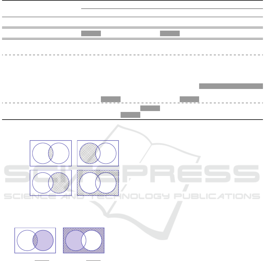
Table 2: The classiﬁcation costs, C for different balancing techniques and feature sets.

Balancing techniques Classiﬁcation cost, C

1,2

, C

1,2

, C

1,2

, C

1,2

IB 0.3267 0.1950 0.2225 0.4008 0.2550 0.2275 0.1992 0.2142 0.2025

OS 0.1708 0.1750 0.1567 0.4025 0.2050 0.2133 0.1867 0.1592 0.1742

OS 0.3467 0.1833 0.2233 0.4167 0.2833 0.2508 0.2083 0.2125 0.2142

SMOTE 0.3100 0.1892 0.2133 0.3658 0.2825 0.2317 0.1875 0.2192 0.2175

Random Under-Sampling (RUS) 0.2733 0.1625 0.2075 0.3817 0.2375 0.1750 0.1525 0.1750 0.1317

TL 0.3475 0.1908 0.2417 0.4233 0.2483 0.2208 0.2025 0.2575 0.2000

Clustering Under-Sampling 0.2408 0.1817 0.1608 0.3992 0.2700 0.1817 0.1725 0.1833 0.1658

NM1 0.3067 0.1658 0.1600 0.3900 0.2700 0.2083 0.1617 0.1608 0.1517

NM2 0.2883 0.1575 0.1583 0.3475 0.3192 0.2775 0.1467 0.1350 0.1258

NM3 0.2050 0.1517 0.1683 0.3342 0.2350 0.1833 0.1725 0.1700 0.1608

Neighborhood Cleaning Rule (NCR) 0.2958 0.1500 0.1617 0.3233 0.2067 0.1717 0.1558 0.1650 0.1558

SMOTE+ENN 0.2492 0.1650 0.1617 0.2875 0.2142 0.2017 0.1575 0.1675 0.1958

SMOTE+TL 0.2550 0.1675 0.1517 0.3283 0.2067 0.2125 0.1617 0.2033 0.1375

Actual Class

A+ A-

Predicted Class

P+

−

P-

−

(a) Confusion matrix with truly and falsely positive

samples detected (TP, FP) in the ﬁrst row, from left to

right and the falsely and truly negative samples detected

(FN, TN) in the second row, from left to right.

−

SE =

T P

T P+F N

−

SP =

T N

T N+FP

(b) Sensitivity and Speciﬁcity evaluation, cor-

responding to the ratio of the doted area over

the blue area.

Figure 5: Evaluation metrics: (a) confusion matrix, (b) Sen-

sitivity - Speciﬁcity.

highlighted in the shaded cells. Table 2 shows the

obtained cost value for each conﬁguration. Strategies

with low cost function are synonymous with a better

SE and SP trade-off.

The obtained results indicate that balancing tech-

niques are essential and improve the classiﬁcation

performance. For this case study the US techniques

and their combination with OS techniques outper-

form the OS techniques. Due to the characteristics

similarities of melanoma and dysplastic lesions, it

is expected to have correlated feature space among

melanoma and dysplastic lesions. Subsequently, the

miss-leading samples could be removed using US and

lead to better performance. Speciﬁcally to our pur-

pose, NM2 algorithm with the combination of all the

features (T

1,2

) with the lowest cost value, achieve

the highest SE and SP of 91.2% and 81.7%. Using the

same feature combination, RUS achieve the second

lowest cost with SE and SP of 92.5% and 78.3%, re-

spectively. The NM2 algorithm also achieve the third

lowest cost with combination of Gabor and color fea-

tures (T

, C

1,2

) with SE and SP of 92.5% and 77.5%,

respectively. Focusing only on OS techniques, OS in

data space outperforms the techniques performing in

feature space.

Comparing the color features, opponent color an-

gle and hue histogram feature descriptor, C

, has a

better performance than well-used color statistics, C

In texture domain, Gabor descriptor, T

, outperforms

CLBP features, T

. Finally, the combination of color

and texture features outperforms any other feature

combination.

6 CONCLUSION

In this paper, we analyzed the impact of data bal-

ancing techniques for the classiﬁcation of malignant

melanoma. Therefore, we presented an extensive

comparison of twelve OS and US techniques in both

feature and data space. These techniques were evalu-

ated on the only public dermoscopic dataset, the PH

BIOIMAGING 2016 - 3rd International Conference on Bioimaging

dataset, in order to provide a chance for future com-

parison. The obtained results particularly highlight

the advantage of balancing the training set over using

the original data, particularly for the methods based

on US (NM2, NCR) and combination of OS and US in

feature space. Furthermore, OS in data space outper-

forms the techniques performing in the feature space.

This study also showed that combining color and tex-

ture features will lead to better performance.

REFERENCES

Abbasi, N. R., Shaw, H. M., et al. (2004). Early diagnosis

of cutaneous melanoma: revisiting the abcd criteria.

Jama, 292(22):2771–2776.

American-Cancer-Society (2014). Cancer facts & ﬁgures

2014.

Barata, C., Marques, J. S., and Emre Celebi, M. (2013).

Towards an automatic bag-of-features model for the

classiﬁcation of dermoscopy images: The inﬂuence of

segmentation. In Image and Signal Processing and

Analysis (ISPA), 2013 8th International Symposium

on, pages 274–279. IEEE.

Barata, C., Ruela, M., Francisco, M., Mendonc¸a, T., and

Marques, J. (2014). Two systems for the detection of

melanomas in dermoscopy images using texture and

color features. IEEE Systems Journal,, 8(3):965–979.

Batista, G. E., Bazzan, A. L., and Monard, M. C. (2003).

Balancing training data for automated annotation of

keywords: a case study. In WOB, pages 10–18.

Batista, G. E., Prati, R. C., and Monard, M. C. (2004). A

study of the behavior of several methods for balancing

machine learning training data. ACM Sigkdd Explo-

rations Newsletter, 6(1):20–29.

Breiman, L. (2001). Random forests. Machine learning,

45(1):5–32.

Capdehourat, G., Corez, A., Bazzano, A., and Mus

e, P.

(2009). Pigmented skin lesions classiﬁcation using

dermatoscopic images. In Progress in Pattern Recog-

nition, Image Analysis, Computer Vision, and Appli-

cations, pages 537–544. Springer.

Celebi, M. E., Kingravi, H. A., et al. (2007). A method-

ological approach to the classiﬁcation of dermoscopy

images. Computerized Medical Imaging and Graph-

ics, 31(6):362–373.

Chawla, N. V., Bowyer, K. W., Hall, L. O., and Kegelmeyer,

W. P. (2002). Smote: synthetic minority over-

sampling technique. Journal of artiﬁcial intelligence

research, pages 321–357.

Forsea, A., Del Marmol, V., de Vries, E., Bailey, E., and

Geller, A. (2012). Melanoma incidence and mortal-

ity in europe: new estimates, persistent disparities.

British Journal of Dermatology, 167(5):1124–1130.

Guo, Z. and Zhang, D. (2010). A completed modeling of

local binary pattern operator for texture classiﬁcation.

IEEE Transactions on Image Processing, 19(6):1657–

1663.

He, H., Garcia, E., et al. (2009). Learning from imbalanced

data. Knowledge and Data Engineering, IEEE Trans-

actions on, 21(9):1263–1284.

Laurikkala, J. (2001). Improving identiﬁcation of difﬁ-

cult small classes by balancing class distribution.

Springer.

Mani, I. and Zhang, I. (2003). knn approach to unbalanced

data distributions: a case study involving information

extraction. In Proceedings of Workshop on Learning

from Imbalanced Datasets.

Prati, R. C., Batista, G. E., and Monard, M. C. (2009). Data

mining with imbalanced class distributions: concepts

and methods. In IICAI, pages 359–376.

Rastgoo, M., Garcia, R., Morel, O., and Marzani, F.

(2015a). Automatic differentiation of melanoma from

dysplastic nevi. Computerized Medical Imaging and

Graphics, 43:44–52.

Rastgoo, M., Morel, O., Marzani, F., and Garcia, R.

(2015b). Ensemble approach for differentiation of ma-

lignant melanoma. In The International Conference

on Quality Control by Artiﬁcial Vision 2015, pages

953415–953415. International Society for Optics and

Photonics.

Tomek, I. (1976). Two modiﬁcations of cnn. IEEE Trans.

Syst. Man Cybern., 6:769–772.

Van De Weijer, J. and Schmid, C. (2006). Coloring local

feature extraction. In Computer Vision–ECCV 2006,

pages 334–348. Springer.

Tackling the Problem of Data Imbalancing for Melanoma Classiﬁcation