A New Parametric Description for Line Structures in 3D Medical Images
by Means of a Weighted Integral Method
Hidetoshi Goto, Takumi Naito and Hidekata Hontani
Dept. of Computer Science and Engineering, Nagoya Institute of Technology, Nagoya, Aichi, 466–8555 Japan
Keywords:
Line Structure Description, Parameter Estimation Problem, Weighted Integral Method.
Abstract:
The authors propose a method that describes line structures in given 3D medical images by estimating the
values of model parameters: A Gaussian function is employed as the model function and the values of the
parameters are estimated by means of a weighted integral method, in which you can estimate the parameter
values by solving a system of linear equations of parameters which are derived from differential equations
that are satisfied by the Gaussian model function. Different from many other model-based methods for the
description, the proposed method requires no parameter sweep and hence can estimate the parameter values
efficiently. Once you estimate the parameter values, you can describe the location, the orientation and the
scale of line structures in given 3D images. Experimental results with artificial 3D images and with clinical
X-ray CT ones demonstrate the estimation performance of the proposed method.
1 INTRODUCTION
In this article, the authors propose a method that
accurately and efficiently describes local line struc-
tures in 3D medical images. The description explic-
itly denotes the location, orientation, and thickness
(scale) of each line structure in given 3D images and
is needed for automatically detecting and analyzing
anatomical vessels or tubes of patients in computer
aided diagnosis systems: Global structures of curves
such as the blood vessels or the bronchi are often
extracted from given images through multiple stages
and you describe the local line structures at the very
first stage in the curve structure extraction (Papari and
Petkov, 2011). For example, active contour models
(Kass et al., 1988) or active shape models (Cootes
et al., 1995) are often employed for extracting curve
structures and they require edge detection before the
models are registered. Edges are generally detected
by local operators and the performance of an edge de-
tector is often evaluated by the accuracy of the de-
tected edges. Not only the locations but also the di-
rections of edges should be accurately described when
you employ Euler curves for describing curve struc-
tures in given images (Kimia et al., 2003; Tamrakar
and Kimia, 2007). In (Engan et al., 1999), the blur-
ring scales of edges also play a very important role
for describing curve structures in images. The accu-
rate information of the location, the orientation, and
the scale helps to group the described local line struc-
tures into the description of global ones.
One of the most major foundations for describing
local line structures, especially for estimating their
scales, can be found in a conventional scale-space
analysis (Lindeberg, 1994; Lindeberg, 1998), which
supplies a theoretical background of the scale selec-
tion in the computation of the SIFT key-points (Lowe,
1999; Lowe, 2004). In the scale-space analysis, you
blur a given image by Gaussian filters with various
scales and estimate the location and the scale (size) of
each structure in the image by observing the change
of image features with respect to the blurring scale
change. Spatial image derivatives that are normal-
ized with respect to the blurring scale are employed
for the image features. A ridge detection method
proposed by Lindeberg (Lindeberg, 1998), for exam-
ple, estimates the location and the scale of each ridge
structure based on a ridge-strength feature computed
from the scale-normalized second derivatives: The
method firstly blurs a given image at various scales
to obtain a set of images blurred at different scales,
then detects center points of ridge structures based on
the first spatial derivatives and computes the ridge-
strength feature at each of the detected center points.
The locations and the scales of ridge structures in the
given image are finally detected by extracting the de-
tected center points at which the ridge-strength fea-
ture is locally maximum with respect to the blurring
208
Goto, H., Naito, T. and Hontani, H.
A New Parametric Description for Line Structures in 3D Medical Images by Means of a Weighted Integral Method.
DOI: 10.5220/0005726602080217
In Proceedings of the 11th Joint Conference on Computer Vision, Imaging and Computer Graphics Theory and Applications (VISIGRAPP 2016) - Volume 4: VISAPP, pages 208-217
ISBN: 978-989-758-175-5
Copyright
c
 2016 by SCITEPRESS – Science and Technology Publications, Lda. All rights reserved

scale change. It should be noted that the scales of the
structures are estimated by detecting the local maxi-
mum of the ridge-strength feature and that the maxi-
mum points are detected by sweeping the scale-space.
Not only the method (Lindeberg, 1998) but also many
other methods (e.g. (Zhu et al., 2010; Si and Zhu,
2012)) estimate the values of the model parameters by
sweeping a parameter space. This means the parame-
ter values estimated by those methods are essentially
quantized and you need to sample the parameter space
more densely in order for improving the accuracy of
the parameter estimation. Steerable filters (Freeman
and Adelson, 1991) are also widely used for describ-
ing local line structures especially for estimating their
directions. You can continuously rotate the direction
of a steerable filter with varying the value of a pa-
rameter and can estimate the direction by referring to
the change of the filter response with respect to the
parameter value: Steerable filter-based methods also
require the sweep of the parameter space. Curvelets
(Starck et al., 2002; Woiselle et al., 2011), Wavelets
(Chuang and Kuo, 1996), and Gabor filters (Zhu et al.,
2010; Si and Zhu, 2012) are also often employed for
describing curves or ridges and their representation of
line features are essentially discretized. Eigen vectors
of a Hessian (Sato et al., 1998) can estimate the line
directions in a continuous way but additional opera-
tions are required for accurately estimating the center
location of a line structure.
The proposed method, on the other hand, can es-
timate the location, orientation, and size of each line
structure without sweeping a parameter space. Anal-
ogous to the scale-space analysis (Lindeberg, 1994;
Lindeberg, 1998), the proposed method employs a
Gaussian function for representing a line structure in a
given image and describes the structure by estimating
the values of the parameters of the Gaussian function
so that the resultant Gaussian function fits to the local
line structure. For the estimation, the authors employ
a weighted integral method (Ando and Nara, 2009),
which was developed for estimating the temporal fre-
quencies of one-dimensional signals.
Given a signal, a weighted integral method esti-
mates the values of the parameters of a model func-
tion by solving a linear system in the parameters,
which is derived from differential equations that are
satisfied by the model function. No parameter sweep-
ing is needed and the values obtained by the method
are essentially quantization-free. The contributions
of this article are as follows: The weighted inte-
gral method is formulated for the analysis of 3D im-
ages for the first time and its description performance
is evaluated using artificial images and medical CT
ones.
µ
0u v
w
3
v
2
v
1
v
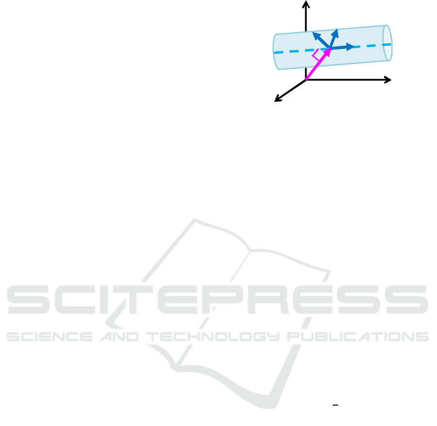
Figure 1: Parameters to be estimated for the description of
a line structure.
2 WEIGHTED INTEGRAL
METHOD FOR 3D IMAGES
Employing a Gaussian function, the proposed method
estimates the parameters of the function for describ-
ing given local appearances by means of a weighted
integral method.
2.1 Notation
Let a three-vector, x
x
x = (x,y,z)
T
, denote the coordi-
nates in a given image and let Ω(x
x
x) denote a local
cubic area in a given image of which center is located
at x
x
x. Let u
u
u = (u, v,w) (−W ≤ u,v,w ≤ +W) denote
the local coordinates in Ω(x
x
x) where the origin is lo-
cated at x
x
x and let I
Ω
(u
u
u) denote an image appearance
in Ω(x
x
x).
In the proposed method, a Gaussian model func-
tion, shown in Eq. (1) is employed for describing a
local image appearance.
f(u
u
u|A,µ
µ
µ,Σ) = Aexp

−
1
2
(u
u
u− µ
µ
µ)
T
Σ
−1
(u
u
u− µ
µ
µ)

,
(1)
where µ
µ
µ and Σ denote the mean vector and the covari-
ance matrix of the Gaussian function, respectively,
and a scalar, A, denotes the magnitude of the function.
Let the eigenvalues of Σ be denoted by λ
i
(i = 1,2,3)
sorted in decreasing order and let the corresponding
eigenvectors be denoted by v
v
v
i
. Let assume that a
line structure is observed in Ω(x
x
x) and that the line
structure is described by a Gaussian function. Then,
λ
1
≃ λ
2
≫ λ
3
≃ 0 and the line direction is parallel
to v
v
v
3
. The location of the line structure in Ω can be
described by µ
µ
µ (See Fig. 1).
For the estimation of the parameters, µ
µ
µ and Σ, we
rewrite f(·|·) in (1) as follows:
f(u
u
u|A
′
,θ
θ
θ) = A
′
exp
(
∑
α,β,γ
θ
αβγ
u
α
v
β
w
γ
)
. (2)
A New Parametric Description for Line Structures in 3D Medical Images by Means of a Weighted Integral Method
209

Here, α,β,γ ∈ {0, 1,2} and 1 ≤ α + β + γ ≤ 2. θ
αβγ
denote the coefficients of u
α
v
β
w
γ
and A
′
denotes the
magnitude. θ
θ
θ = (θ
αβγ
)
T
is a nine-vector. Given a lo-
cal image, I
Ω
(u
u
u), the proposed method estimates the
values of the nine parameters, θ
θ
θ, in (2) by using a
weighted integral method, of which details are de-
scribed in the next subsection. It is straightforward
to compute µ
µ
µ and Σ in (1) from θ
θ
θ.
2.2 Weighted Integral Method
Given a signal, a weighted integral method (Ando and
Nara, 2009; Goto and Hontani, 2013) estimates the
values of the parameters of a model function for fit-
ting the model to the given signal. The values are
estimated not by sweeping the space of the parame-
ters but by solving a system of linear equations of the
parameters, which is derived from a set of differential
equations that the model function satisfies.
The Gaussian function f(u
u
u|·) in (2) satisfies the
following differential equation at every location, u
u
u:
∂f(u
u
u|·)
∂u
=
∑
α,β,γ
θ
α,β,γ
u
α−1
v
β
w
γ
f(u
u
u|·). (3)
Let ∂
u
α
v
β
w
γ
f(u
u
u|·) be denoted by f
u
α
v
β
w
γ
(u
u
u|·). It
should be noted that, when a local image, I
Ω
(u
u
u), is
given, the derivatives of f
u
α
v
β
w
γ
(u
u
u|·) in (3) are known
and the differential equation in (3) is just a linear
equation of the parameters, θ
αβγ
. By differentiating
f(u
u
u|·) with v and w, you obtain other linear equa-
tions of θ
θ
θ, and the proposed method estimates the val-
ues of θ
θ
θ by solving the system of these linear equa-
tions. The values of the derivatives in these equa-
tions, though, are easily perturbed by image noises
and hence the weighted integral method converts the
differential equations into integral ones for estimating
the parameter values more stably against the noises.
Let c(u
u
u) denote a weight function defined on the
local region, Ω(x
x
x). The following equation holds for
any weight function because the linear equation (3)
holds at every location in Ω(x
x
x):
Z
Ω
(
f
u
(u
u
u) −
∑
α,β,γ
θ
α,β,γ
u
α−1
v
β
w
γ
f(u
u
u)
)
c(u
u
u)du
u
u = 0.
(4)
You can rewrite (4) as follows:
Z
Ω
f
u
(u
u
u)c(u
u
u)du
u
u−
∑
α,β,γ
g
(α−1)βγ
θ
αβγ
= 0, (5)
where
g
αβγ
≡
Z
Ω
u
α
v
β
w
γ
f(u
u
u)c(u
u
u)du
u
u. (6)
The values of g
αβγ
in (6) can be computed more stably
against the noises than the values of the derivatives,
f
u
α
v
β
w
γ
, because of the spatial integration. By apply-
ing the partial integration to the first term of the left
hand side of (5), you obtain the following equation:
Z
Ω
f
u
(u
u
u)c(u
u
u)du
u
u = [ f(u
u
u)c(u
u
u)]
Ω
−
Z
Ω
f(u
u
u)
∂c(u
u
u)
∂u
du
u
u.
(7)
You can eliminate the first term of the right hand side
of (7) if you employ a weight function such that
c(u
u
u) = 0 if u
u
u ∈ ∂Ω(x
x
x), (8)
where ∂Ω(x
x
x) denotes the boundary of the region,
Ω(x
x
x). In the proposed method, we hence employ the
Hann window function for constructing c(u
u
u):
c(u
u
u|ω
ω
ω) = p(u)p(v)p(w)e
− j(ω
ω
ω
T
u
u
u)
, (9)
where ω
ω
ω = (ω
u
,ω
v
,ω
w
)
T
denotes the frequencies of
the complex sinusoidal function appeared in the right
hand side and p(·) denotes the Hann window func-
tion,
p(u) =
1
2

1+ cos

πu
W

. (10)
The weight function (9) satisfies the condition shown
in (8) and now the first term of the left hand side of
(7) has an expression as follows:
Z
Ω
f
u
(u
u
u)c(u
u
u)du
u
u = −
Z
Ω
f(u
u
u)
∂c(u
u
u)
∂u
du
u
u. (11)
Using the expression shown in the right hand side
of (11), you can compute the value of the integra-
tion more accurately because you can compute the
value of c
u
(u
u
u) analytically: No finite difference ap-
proximation is needed for computing the values of the
derivatives. As a result, from the weighted integral of
f
u
(u
u
u|·) shown in (7), you obtain one following com-
plex linear equation:
− jω
u
g
000
+ h
u
−
∑
α,β,γ
θ
αβγ
g
(α−1)βγ
= 0, (12)
where
h
u
≡
Z
Ω
f(u
u
u)
∂p(u)
∂u
p(v)p(w)e
− j(ω
ω
ω
T
u
u
u)
du
u
u. (13)
Analogously, using an identical weight function,
you can obtain other complex equations from the
derivatives, f
v
(u
u
u|·) and f
w
(u
u
u|·), such that
− jω
v
g
000
+ h
v
−
∑
α,β,γ
θ
αβγ
g
α(β−1)γ
= 0, (14)
− jω
w
g
000
+ h
w
−
∑
α,β,γ
θ
αβγ
g
αβ(γ−1)
= 0. (15)
Each of the linear equations consists of two equations
that correspond to the real part and the imaginary one
and hence you can obtain 3 × 2 = 6 different linear
VISAPP 2016 - International Conference on Computer Vision Theory and Applications
210

equations of the parameters shown in (12), (14), and
(15) by computing the weighted integrals.
Having nine unknowns, you need more than nine
independent linear equations for estimating the pa-
rameter values uniquely. In the experiments, four dif-
ferent weight functions each of which corresponds to
the different frequencies, ω
ω
ω
(k)
(k = 0, 1,2, 3) are used
for obtaining enough number of independent linear
equations and the parameter values are estimated by
solving the system of 24 linear equations such that




A
(0)
A
(1)
A
(2)
A
(3)




θ
θ
θ =





b
b
b
(0)
b
b
b
(1)
b
b
b
(2)
b
b
b
(3)





, (16)
where
A
(k)
=








g
100
R
0 0 g
010
R
0 g
001
R
g
000
R
0 0
g
100
I
0 0 g
010
I
0 g
001
I
g
000
I
0 0
0 g
010
R
0 g
100
R
g
001
R
0 0 g
000
R
0
0 g
010
I
0 g
100
I
g
001
I
0 0 g
000
I
0
0 0 g
001
R
0 g
010
R
g
100
R
0 0 g
000
R
0 0 g
001
I
0 g
010
I
g
100
I
0 0 g
000
I








(17)
and
b
b
b
(k)
=









−h
u
R
− ω
u
g
000
I
−h
u
I
+ ω
u
g
000
R
−h
v
R
− ω
v
g
000
I
−h
v
I
+ ω
v
g
000
R
−h
w
R
− ω
w
g
000
I
−h
w
I
+ ω
w
g
000
R









. (18)
both of which are obtained by using the weight func-
tion, c(u
u
u|ω
ω
ω
(k)
). Here, g
R
and g
I
denote the real part
and the imaginary part of the complex number, g.
2.3 Weight Function
As described above, different weight functions are
used in the computation of g
αβγ
, h
u
, h
v
, and h
w
shown
in (17) and (18) in order for obtaining enough num-
ber of linear equations. Different weight functions are
constructed by changing the frequencies, ω
ω
ω. In the ex-
periments reported in the next section, we set
ω
(k)
u
=
πn
(k)
u
W
, ω
(k)
v
=
πn
(k)
v
W
, ω
(k)
w
=
πn
(k)
w
W
, (19)
where (n
(k)
u
,n
(k)
v
,n
(k)
w
) = (+1,+1, +1), (+1,+1,−1),
(+1,−1,+1), (−1, +1,+ 1) for k = 0,1, 2,3, respec-
tively. Figure 2 shows a weight function, c(u
u
u|ω
ω
ω
(0)
).
Real part Imaginary part
Figure 2: Profiles of the weight function, c(u
u
u|ω
ω
ω
(0)
).
2.4 Automatic Window Size Selection
In the proposed method, the size of window, Ω(x
x
x),
is adaptively selected at each location. As men-
tioned above, the coefficients of the linear systems
(16) are computed by integrating the weighted ap-
pearances in Ω. Let the side length of Ω be denoted
by L (= 2W + 1) (see Sec. 2.1). The accuracy of the
weighted integral method depends on the sizes of the
windows in which the weighted appearances are inte-
grated for computing the coefficients, g
αβγ
, h
u
, h
v
, and
h
w
, in the linear systems (16) (you will see details in
Sec. 3.1). When the window sizes are too small, the
estimation is more sensitive to measurement noises.
Too large windows, on the other hand, often degrade
the accuracy because neighboring structures are often
included in a single window and because the resultant
appearance in the window cannot be described by the
model function. Hence, you need to determine an ap-
propriate size of the window at each location in given
images for making the parameter estimation more ac-
curate. The authors propose a new method that adap-
tively selects the appropriate window size from a set
of candidate sizes for each location in given images.
As mentioned above, the weighted integral method
solves the systems of linear equations with respect to
the parameters. The proposed method selects a win-
dow size by evaluating the uniqueness of the solution
of (16). It should be noted that, though the window
sizes determined by the proposed method are quan-
tized, the estimated values of the parameters are not
quantized at all.
Let the candidates of the window sizes be de-
noted by L
(0)
, L
(1)
,... , L
(M)
, where M + 1 denotes
the total number of the candidates and L
(m−1)
< L
(m)
(m = 1, 2,.. .,M). Let L
(m)
× L
(m)
window centered
at x
x
x be denoted by Ω
(m)
(x
x
x) and let the system of the
linear equations (16) obtained with Ω
(m)
(x
x
x) be de-
noted by A
(m)
θ
θ
θ = b
b
b
(m)
. The proposed method selects
an appropriate window size from the set, {L
(m)
|m =
0,1, ..., M}, by quantitatively evaluating the unique-
ness of the solution of the linear system, A
(m)
θ
θ
θ = b
b
b
(m)
.
The linear system (16) can be rewritten as follows:
A New Parametric Description for Line Structures in 3D Medical Images by Means of a Weighted Integral Method
211

[A − b
b
b]θ
θ
θ
′
= 0, (20)
where θ
θ
θ
′
= [θ
θ
θ|1]
T
. Let A
′
= [A| − b
b
b]. Then, the rank
of the 24 × 10 matrix, A
′
, should be equal to nine,
i.e. rank(A
′
) = 9, if (20) has a unique solution. Let
the singular values of A
′
be denoted by s
′
1
,s
′
2
,... ,s
′
10
,
where s
′
n
≥ s
′
n+1
(n = 1,2,.. .,9). We evaluate the
uniqueness of the solution of (16) as follows:
F(A,b
b
b) =
s
′
10
s
′
9
. (21)
Note that rank(A
′
) = 9 when the local appearance in
Ω exactly fits the model function (1): s
′
9
> 0 and
s
′
10
= 0, i.e., the proposed criterion, F(·,·), is equal
to zero. The proposed method, hence, judges that the
local appearance in Ω is suitable for the parameter es-
timation when the values of F are close to zero.
At each location, x
x
x, the proposed method selects
the window size L(x
x
x) that minimizes F(A
(m)
,b
b
b
(m)
) for
computing the coefficients of the linear equations.
L(x
x
x) = arg min
m=0,1,...,M
F(A
(m)
,b
b
b
(m)
). (22)
The candidates of the window sizes are determined as
follows. Let a range of the scales that should be ac-
curately estimated be denoted by T
σ
= {σ|σ
min
≤ σ ≤
σ
max
}, where σ
min
and σ
max
are the minimum scale
and the maximum one to be accurately estimated, re-
spectively. Let a range of the scale that can be accu-
rately estimated by using the window Ω
(m)
be denoted
by R
(m)
σ
, where R
(m)
σ
= [αL
(m)
,βL
(m)
] and 0 < α < β.
The candidates of the window sizes should be deter-
mined so that the following condition is satisfied:
T
σ
⊆
M
[
m=0
R
(m)
σ
. (23)
In the proposed method, the minimum window size,
L
(0)
, is firstly determined so that the minimum scale
is in the range R
(0)
σ
, i.e., αL
(0)
≤ σ
min
(≤ βL
(0)
). Us-
ing the smallest window Ω
(m)
, you can accurately es-
timate the scales between αL
(0)
and βL
(0)
. The size
of the second smallest window is then determined so
that the upper boundary scale, βL
(0)
, can be accu-
rately estimated not only with the window Ω
(0)
but
also with Ω
(1)
, i.e., αL
(1)
≤ βL
(0)
. In the proposed
method, we determine the second smallest window
size so that R
(1)
σ
overlaps with the one quarter of R
(0)
σ
,
i.e. αL
(1)
= (α + 3)L
(0)
/4. Analogously, we deter-
mine all of the window sizes as follows:
L
(m)
= ρ
m
L
(0)
, (24)
where ρ = (α+ 3)/(4α) in the proposed method. The
value of the coefficient, ρ, varies depending on the
ratio of the overlaps between R
(m)
σ
and R
(m+1)
σ
. The
total number of the candidates, M, is determined so
that σ
max
can be accurately estimated using the largest
window L
(M)
, i.e. σ
max
< βL
(M)
. Setting m = M, the
equation (24) can be rewritten as follows:
ρ
M
=
L
(M)
L
(0)
>
ασ
min
βσ
max
. (25)
You can determine the total number of the candidates
M as follows:
M =
&
log
ρ
L
(M)
L
(0)
'
=

log
ρ
ασ
max
βσ
min

. (26)
For example, when α = 1/6, β = 1/4, σ
min
= 2.0,
σ
max
= 20.0, then we obtain M = 6. Not so many
candidates are needed for covering a wide range of
the scales.
3 EXPERIMENTS
3.1 Experiments with Artificial Images
Randomly sampling the parameter values of the
Gaussian function, we firstly generated a set of noise-
free images of a line structure and then added Gaus-
sian noises to the images for obtaining a set of noisy
ones. Applying the proposed method to the images,
we evaluated the accuracy of the parameter estima-
tion of the proposed method.
As described in Sec. 2.1, the eigenvector of the
covariance matrix shown in (1) that has the minimum
eigenvalue represents the direction of a target line. Let
¯
v
v
v denote the true direction and let
ˆ
v
v
v denote the di-
rection computed from the estimated covariance ma-
trix. For the evaluation, the window size was fixed as
W = 10 pixel and the scale of the lines in the artifi-
cial images was set as
¯
σ = 5.0. The direction vectors,
¯
v
v
v, were randomly generated under the condition that
kv
v
vk = 1. Figure 3 shows some examples of the ar-
tificial images with different SN ratios. Firstly, the
accuracy of the estimation the line direction was eval-
uated. The proposed method estimates the values of
the parameters, θ
α,β,γ
, and you can straightforwardly
compute the line direction v
v
v
3
shown in Fig. 1. Here,
v
v
v
3
is a unit 3-vector and can be represented by a sin-
gle point on a unit sphere. Let the true direction of the
line in a given image be denoted by
ˆ
v
v
v and let the point
of the unit sphere corresponding to
ˆ
v
v
v be denoted by
ˆ
V.
We represented the distribution of the estimated direc-
tions,
ˆ
v
v
v
3
, from the synthesized images by the points
on the unit sphere and these points were projected on
the tangent plane to the unit sphere at
ˆ
V. The resul-
tant distributions observed at different SN ratios are
VISAPP 2016 - International Conference on Computer Vision Theory and Applications
212

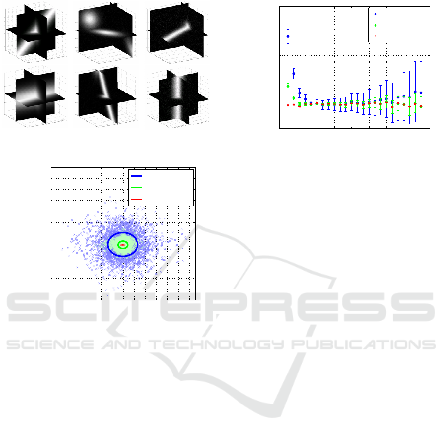
SNR = ∞ dB SNR = 40 dB
SNR = 20 dB
Figure 3: Examples of the artificial 3D images.
−0.06 −0.03 0.00 0.03 0.06
−0.04
−0.02
0.00
0.02
0.04
0.06
direction along e_0 [rad]
direction along e_1 [rad]
SNR=20dB
SNR=40dB
SNR=∞ dB
Figure 4: Experimental results of the estimation of the di-
rections.
demonstrated in Fig. 4. The red, green and blue dots
correspond to the estimated directions from the im-
ages with the SN ratio = ∞, 40, and 20 dB, respec-
tively. As shown in the figure, the estimation error
variance increased with respect to the decrease of the
SN ratio but the estimation was unbiased: The center
of the dots was identical with the true direction.
Then, for evaluating the accuracy of the scale esti-
mation, a set of the artificial images in which the line
structures have varieties of the scale values was used.
A graph shown in Fig. 5 shows the result. The hor-
izontal axis of the graph indicates the values of the
true scale
¯
σ and the vertical one indicates the ratio of
the estimated scale
ˆ
σ to the true one. As shown in
the graph, when the given images are noise free im-
ages, the proposed method successfully estimated the
scales regardless of the value. When the SN ratio de-
creased, the estimation quality degraded at the smaller
scales (
¯
σ < 2) and at the larger scales (
¯
σ > 6). It
should be noted that these results were obtained with a
fixed window size (L = 2W + 1) and that these results
are useful for determining the values of α and of β,
which determine the range of the scale, R
σ
, in which
2 3 4 5 6 7 8 9
0.98
1
1.02
1.04
1.06
1.08
True value of σ [pixel]
Ratio, r
σ
=σ
estimates
/σ
true
SNR=20dB
SNR=40dB
SNR=∞ dB
Figure 5: Experimental results of the scale estimation.
scales you can accurately estimate with the window
size, L
∗
.
The robustnessof the proposed method, the ability
of the method against input images of which patterns
do not strictly obey the model, is evaluated. In this
article, we report on the results obtained when the in-
put line patterns were represented by a pill-box model
such that
I(x
x
x;σ) =

1, if x
2
+ z
2
< σ
2
,
0, otherwise,
(27)
The estimation performance against non-Gaussian
patterns is improved by firstly blurring the input im-
ages with Gaussian of which scale is σ
2
0
, estimat-
ing the scale,
ˆ
σ
2
using the propose method and out-
putting
ˆ
σ
2
=
ˆ
σ
2
− σ
2
0
. Figure 6 shows the results.
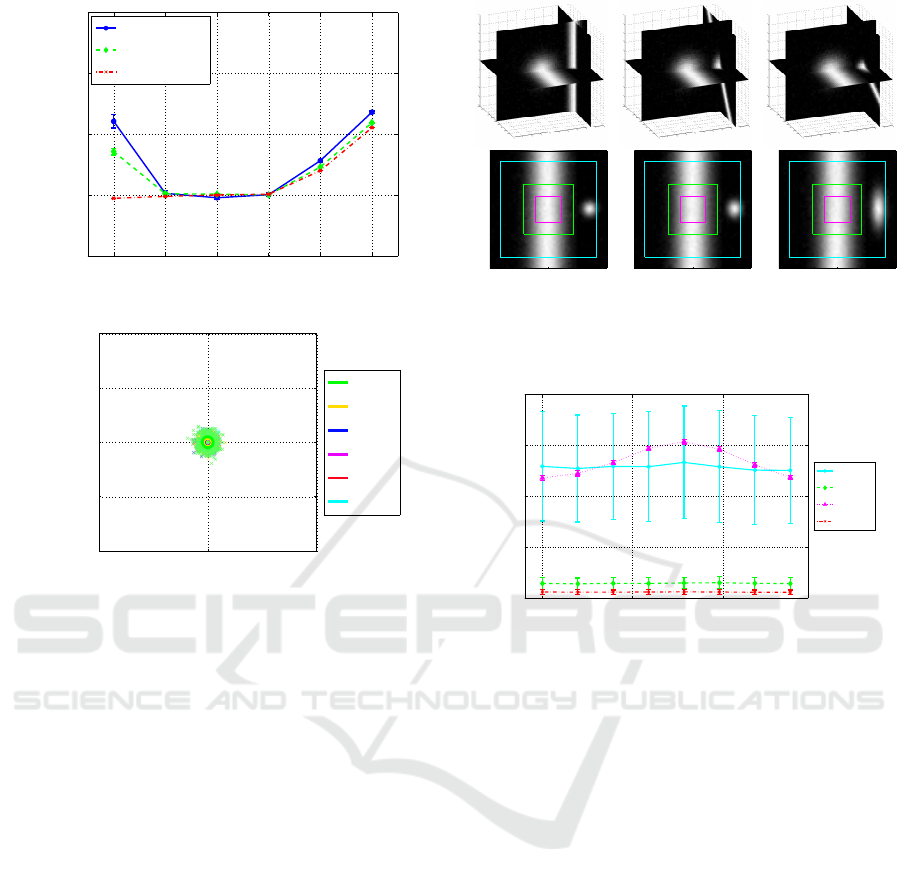
As shown, the proposed method unfortunately under-
estimated the scales, but the estimated scale values
were proportional to the true ones. It should be noted
that the scale space analysis (Lindeberg, 1994; Linde-
berg, 1998), which is one of the most standard method
for the scale estimation, is also biased: When non-
Gaussian patterns are input, the scale-space analysis
outputs biased scales, which are proportional to the
true scales (Lindeberg, 1994). On the other hand, as
shown in Fig. 6(B), the estimated directions of non-
Gaussian line patterns were unbiased.
Then, we evaluated the performance of the win-
dow size selection. As mentioned above, an appropri-
ate windowsize should be selected because a too large
window often includes not only a target line but also
neighboringother structures and fails to accurately es-
timate the parameter values and a too small window
is too sensitive to image noises and fails to accurately
estimate the parameter values. For the evaluation, we
generated two sets of artificial images. One set con-
sists of images of two separate lines with different
directions and the other set consists of images of a
curved line. When multiple lines are included in a
A New Parametric Description for Line Structures in 3D Medical Images by Means of a Weighted Integral Method
213

2 3 4 5 6 7
0.4
0.5
0.6
0.7
0.8
True value of σ [pixel]
Ratio, σ
estimate
/σ
true
SNR=20dB
SNR=40dB
SNR=∞ dB
(A) Scale estimation
−0.02 0 0.02
−0.02
−0.01
0
0.01
0.02
direction along e_0 [rad]
direction along e_1 [rad]
σ=2.0
σ=3.0
σ=4.0
σ=5.0
σ=6.0
σ=7.0
(B) Direction estimation
Figure 6: Experimental results obtained from a set of artifi-
cial images that satisfy the equation (27).
given image, you cannot accurately estimate the pa-
rameters and so you need to automatically select an
appropriate (not too small) windows size so that the
window includes only one single line structure. Top
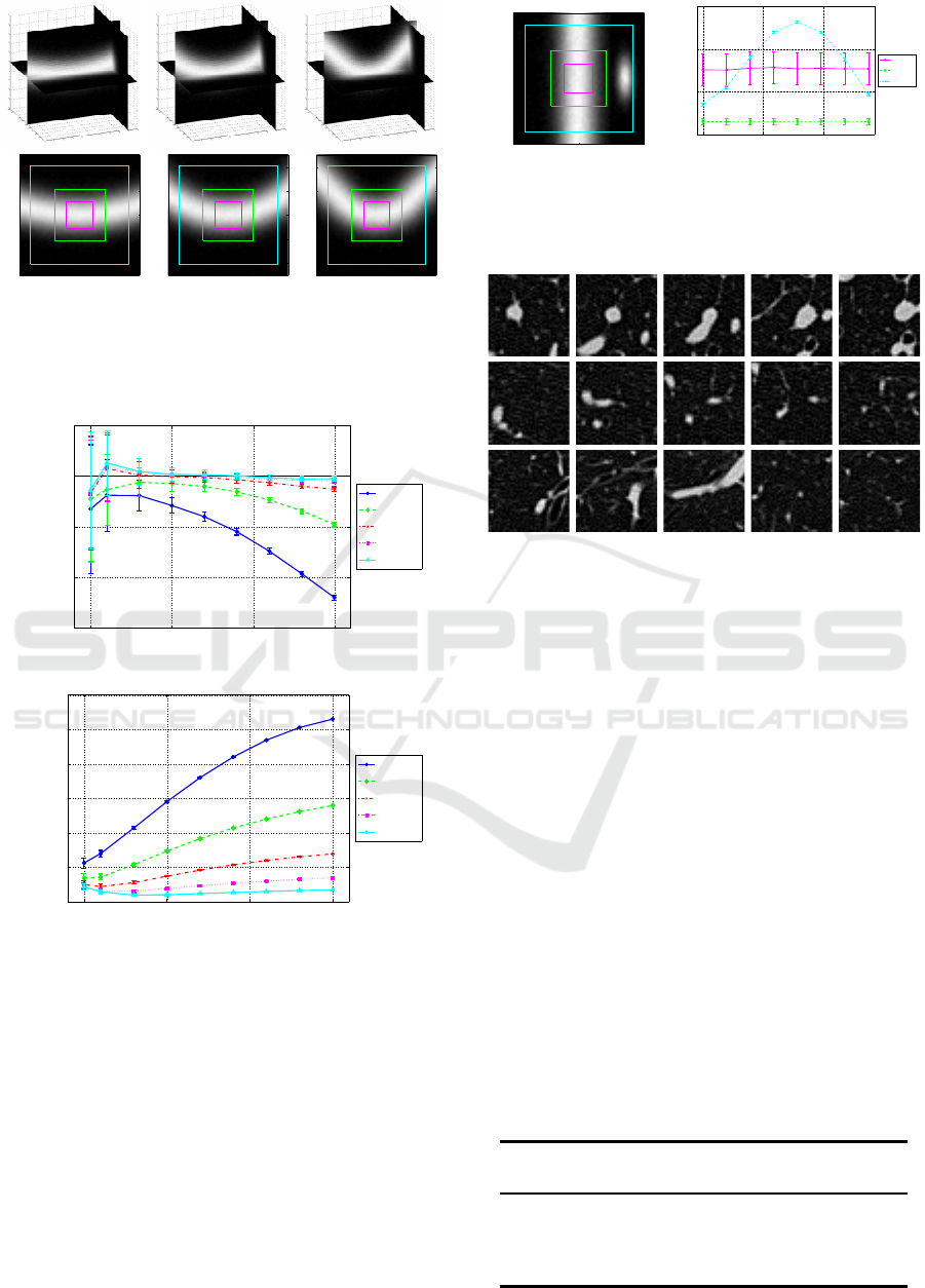
panels in Fig. 7 show some examples of the images
of two lines and the bottom ones show three windows
with different sizes. As shown, when the windows
size is large, the two lines are included in the window.
As shown in Fig. 8, when you automatically select an
appropriate window size at each location in given im-
ages, you obtain more accurate estimations than when
you use fixed size windows. Figure 9 shows exam-
ples in the latter set. As shown, images of curves
with different curvatures are given. When a curve
line is given, the image pattern in the window devi-
ate more largely from a Gaussian straight line model
as the window size is increased. As shown in Fig. 10,
smaller size of windows were selected when the cur-
vatures of the lines were larger and the estimation ac-
curacy was improved by applying the automatic win-
dow size selection. Figure 11 shows an example of
the change of F(A,b
b
b) with respect to the window size.
The left panel of Fig. 11 shows an input image and
thee windows with different sizes and the right panel
shows the value of F computed with the three win-
−20 −10 0 10 20
−20
−10
0
10
20
−20 −10 0 10 20
−20
−10
0
10
20
−20 −10 0 10 20
−20
−10
0
10
20
Figure 7: Examples of the two line structures. The 2D im-
ages in the bottom row show the axial-slice (x-y plane) at
z = 0. The squares in the 2D images indicate the smallest,
the middle, and the largest applied windows.
0 0.5 1
0
2
4
6
8
Angle between 2 lines [rad]
Reconstruction error (RMSE)
W=5
W=10
W=20
WSS
Figure 8: Experimental results of the effects of the window
size selection on the estimation accuracy. In the legend,
WSS means the window size selection.
dows. As shown, the value of F was the smallest
when the window was enough large comparing with
the line width and was enough small so that no neigh-
boring structures was included.
3.2 Experiments with Medical Images
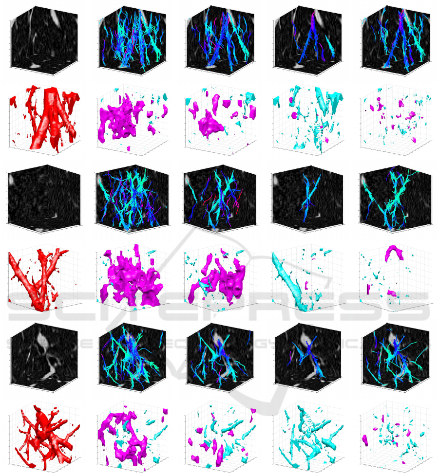
The authors applied the proposed method to a set of
X-ray 3D medical images of the lungs for describing
the structures of the blood vessels. Figure 12 shows
some examples of the input images and Fig. 13 shows
the descriptions obtained by the proposed method.
In Fig. 13, the odd rows shows the results obtained
by the proposed method and the even rows shows
the surface rendering of the differences between the
given images and the results. The second column,
the third one, and the fourth one show the result ob-
tained by the proposed method with the fixed window
size (W = 5,6, 8), respectively, and the right column
shows the results obtained by the proposed method
with the window size selection. In the odd rows in
Fig. 13, the parameter values estimated by the pro-
posed method are indicated by colored line segments:
VISAPP 2016 - International Conference on Computer Vision Theory and Applications
214

−20 −10 0 10 20
−20
−10
0
10
20
r = 80
−20 −10 0 10 20
−20
−10
0
10
20
r = 40
−20 −10 0 10 20
−20
−10
0
10
20
r = 20
Figure 9: Examples of the curve structures. The 2D images
in the bottom row show the coronal-slice (x-z plane) at y =
0. The squares in the 2D images indicate the smallest, the
middle, and the largest applied windows.
10 20 30 40
0.97
0.98
0.99
1
1.01
Window size, L [pixel]
Ratio, σ
estimate
/σ
true
R= 20
R= 40
R= 80
R=160
R=320
(A) Scale estimation
10 20 30 40
0
0.01
0.02
0.03
0.04
0.05
0.06
Window size, L [pixel]
F(A,b)
R= 20
R= 40
R= 80
R=160
R=320
(B) Proposed criterion
Figure 10: Experimental results of the effects of the window
size selection on the estimation robustness.
The location of each segment is determined by the
estimated location, µ
µ
µ, the direction of the segment
is determined by the estimated direction, v
v
v
3
, and the
color of the segment is determined by the estimated
scale. You can reconstruct line structures from these
line segments: Generating a Gaussian that has the es-
timated parameters from each of the segments, you
obtain line structures that have the estimated param-
eter values. We compared this reconstructed images
with the input original ones. Let a reconstructed im-
age be denoted by I
re
and let the corresponding input
−20 −10 0 10 20
−20
−10
0
10
20
Input images
0 0.5 1
0
0.005
0.01
0.015
Angle between 2 lines [rad]
F(A,b)
W=5
W=10
W=20
Proposed criterion, F(A, b
b
b)
Figure 11: Experimental results of the proposed criterion,
F(A, b
b
b), obtained from the set of the artificial images of two
separate lines.
z = 4 z = 12 z = 20 z = 28 z = 36
Figure 12: Examples of the X-ray CT images of lungs used
in the experiments. Some axial slices are indicated.
image be denoted by I
input
. Let ∆
I
= I
re
−I
input
. To en-
hance the difference, we binarized the difference im-
age ∆
I
and demonstrated binarized images in the even
rows in Fig. 13. In the binarized images, blue color
regions indicate ∆
I
> 0 and the pink regions indicate
∆
I
< 0. As shown in the figures, we obtained more ac-
curate reconstruction when the window size is adap-
tively selected at each image location. As you can see
the figures, our method failed to reconstruct the pat-
terns of non-line structures such as junctions and we
need to implement such the regions by using the line-
structure descriptions. Table 1 shows the mean value
of the over-detection rate and the detection failure rate
for each method when the results shown in Fig. 13
were obtained. As shown, the proposed method with
the window size selection can estimate the values of
the parameters, that describe the line structure at each
location, more accurately and more robustly than the
weighted integral method with the fixed size window.
Table 1: Comparison of the mean among the results shown
in Fig. 13 on the accuracy of the line description.
Over-detec- Detection
Proposed method tion rate failure rate
Fixed as W = 5 27.5 % 6.7 %
Fixed as W = 6 23.0 % 14.5 %
Fixed as W = 8 7.2 % 42.0 %
Window size selection 12.7 % 10.9 %
A New Parametric Description for Line Structures in 3D Medical Images by Means of a Weighted Integral Method
215

Input images Fixed size window Fixed size window Fixed size window Proposed method
Figure 13: Examples of the descriptions obtained from the images shown in Fig. 12. The columns from second to fifth show
the results by the proposed method with the fixed size window (W = 5,6,8) and the window size selection, respectively. The
colors in the odd rows indicates the estimated scale, e.g., cool colors indicates thin lines. In the even rows, red, blue, and pink
indicate the regions of I
input
, ∆
I
> 0, and ∆
I
< 0, respectively.
4 CONCLUSIONS
In this article, the authors proposed a new method
that accurately and efficiently estimates the parame-
ters of the Gaussian model for describing local curvi-
linear structures in 3D images. The weighted inte-
gral method linearizes the parameter estimation prob-
lem based on the differential equations satisfied by
the Gaussian model function. The proposed window
size selection determines appropriate windowsizes by
VISAPP 2016 - International Conference on Computer Vision Theory and Applications
216

evaluating whether a solution of the system of the lin-
ear equations exists uniquely. Experimental results
demonstrated that the method estimated accurately
and robustly the parameter values of local curvilinear
structure in given images, and that the estimated val-
ues of parameters obtained the method describe accu-
rately and robustly the curvilinear structures in given
3D medical images.
Future works include to develop a method that
can describe local appearances using the other model
functions that is not the Gaussian function, e.g., the
Gabor function and the wavelet, and that can auto-
matically select an appropriate model function at each
location from a set of the model function.
ACKNOWLEDGEMENTS
This work was supported by JSPS Grant-in-Aid for
Scientific Research on Innovative Areas (Multidis-
ciplinary Computational Anatomy) JSPS KAKENHI
Grant Number, 26108003.
REFERENCES
Ando, S. and Nara, T. (2009). An exact direct method
of sinusoidal parameter estimation derived from finite
Fourier integral of differential equation. IEEE Trans.
Signal Process., 57(9):3317–3329.
Chuang, G. C.-H. and Kuo, C.-C. (1996). Wavelet descrip-
tor of planar curves: theory and applications. IEEE
Trans. Image Process., 5(1):56–70.
Cootes, T., Taylor, C., Cooper, D., and Graham, J. (1995).
Active shape models – their training and application.
Comput. Vis. Image Understanding, 61(1):38 – 59.
Engan, K., Aase, S. O., and H˚akon Husøy, J. (1999).
Method of optimal directions for frame design. In
Proc., IEEE Int’l Conf. Acoustics, Speech, and Signal
Process., volume 5, pages 2443–2446.
Freeman, W. T. and Adelson, E. H. (1991). The design
and use of steerable filters. IEEE Trans. Pattern Anal.
Mach. Intell., 13(9):891–906.
Goto, H. and Hontani, H. (2013). A weighted integral
method for parametrically describing local image ap-
pearance. IPSJ Trans. Comput. Vis. Appl., 5:70–74.
Kass, M., Witkin, A., and Terzopoulos, D. (1988). Snakes:
Active contour models. Int’l J. Comput. Vis., 1(4):
321–331.
Kimia, B. B., Frankel, I., and Popescu, A.-M. (2003). Eu-
ler spiral for shape completion. Int’l J. Comput. Vis.,
54(1-3):159–182.
Lindeberg, T. (1994). Scale-Space Theory in Computer Vi-
sion. Kluwer Academic Publishers.
Lindeberg, T. (1998). Edge detection and ridge detection
with automatic scale selection. Int’l J. Comput. Vis.,
30(2):117–156.
Lowe, D. G. (1999). Object recognition from local scale-
invariant features. In Proc., IEEE Int’l Conf. Comput.
Vis., volume 2, pages 1150–1157.
Lowe, D. G. (2004). Distinctive image features from scale-
invariant keypoints. Int’l J. Comput. Vis., 60(2):91–
110.
Papari, G. and Petkov, N. (2011). Edge and line oriented
contour detection: State of the art. Image Vis. Com-
puting, 29(2-3):79 – 103.
Sato, Y., Nakajima, S., Shiraga, N., Atsumi, H., Yoshida, S.,
Koller, T., Gerig, G., and Kikinis, R. (1998). Three-
dimensional multi-scale line filter for segmentation
and visualization of curvilinear structures in medical
images. Medical Image Anal., 2(2):143–168.
Si, Z. and Zhu, S. (2012). Learning hybrid image templates
(HIT) by information projection. IEEE Trans. Pattern
Anal. Mach. Intell., 34(7):1354–1367.
Starck, J.-L., Cand`es, E. J., and Donoho, D. L. (2002). The
curvelet transform for image denoising. IEEE Trans.
Image Process., 11(6):670–684.
Tamrakar, A. and Kimia, B. B. (2007). No grouping left
behind: From edges to curve fragments. In IEEE Int’l
Conf. Comput. Vis., pages 1–8.
Woiselle, A., Starck, J.-L., and Fadili, J. (2011). 3-D data
denoising and inpainting with the low-redundancy fast
curvelet transform. J. Math. Imaging Vis., 39(2):121–
139.
Zhu, S., Shi, K., and Si, Z. (2010). Learning explicit and
implicit visual manifolds by information projection.
Pattern Recognition Letters, 31(8):667–685.
A New Parametric Description for Line Structures in 3D Medical Images by Means of a Weighted Integral Method
217