A Predictive Model for Smart Control of a Domestic Heat Pump and

Thermal Storage

R. P. van Leeuwen

1,2

, I. Gebhardt

, J. B. de Wit

and G. J. M. Smit

Department of Computer Science, Mathematics and Electrical Engineering, University of Twente,

P.O. Box 217, 7500 AE Enschede, The Netherlands

Sustainable Energy Group, Saxion University of Applied Sciences,

P.O. Box 70.000, 7500 KB Enschede, The Netherlands

Keywords:

Smart Energy Storage, Energy Proﬁling and Measurement, Smart Grid, Optimal Heat Pump Control, Energy

Management Systems, Load Balancing.

Abstract:

The purpose of this paper is to develop and validate a predictive model of a thermal storage which is charged

by a heat pump and used for domestic hot water supply. The model is used for smart grid control purposes

and requires measurement signals of ﬂow and temperature at the inlet and outlet of the storage to determine

charged and discharged thermal energy, and electrical energy consumption of the heat pump. The paper

reviews possible simulation models and describes a predictive model for the state of charge and for the heat

pump power consumption during charging based on experimental data. Simulations are carried out and results

are compared with experiments. The model is applied in a case of domestic smart energy control for which

results are shown.

1 INTRODUCTION

To reduce carbon dioxide emissions, energy supply

systems around the world increasingly integrate en-

ergy from renewable sources such as solar Photo

Voltaic (PV), wind turbines and biomass conversion.

On a local scale of households and small companies

this concerns mainly rooftop solar PV systems, urban

wind turbines and bio-gas Combined Heat and Power

installations (CHP). Due to the daily solar move-

ment, dependence on weather conditions and people’s

consumption patterns, there is a mismatch between

times of energy production and demand. For existing

low voltage grids this can cause voltage increase be-

yond acceptable bounds at times of overproduction or

voltage decrease at times when the demand is much

higher than the local production.

As pointed out in (Nykamp, 2013), an expensive so-

lution is to strengthen the existing grid. An econom-

ically more attractive alternative is to invest in smart

grids. The purpose of a smart grid for a low voltage

network is to balance local electricity production with

demand. A hybrid smart micro grid combines electric

production and demand with thermal energy produc-

tion and demand. The solution contains smart control

of ﬂexible devices (i.e. washing machines, dishwash-

ers, heat pumps) and may also contain electric and

thermal storage. By controlling ﬂexible devices and

storage chargers, grid overloads either due to overpro-

duction or demand peaks are avoided (Leeuwen et al.,

2015).

As only part of the demand is ﬂexible and due to

increased electriﬁcation of household and transporta-

tion energy demand, there is often a high level of si-

multaneous energy demand within an area. Therefore,

electrical and thermal storage systems are gaining im-

portance. To control storage charging and discharg-

ing, algorithms used for smart energy control need

actual information on the state of charge (SoC) of

the storage in order to predict the amount of charg-

ing or discharging which is possible in the near fu-

ture. As most smart control algorithms rely on linear

programming or control heuristics, and our interest is

on application in local embedded systems as part of

the storage, the predictive model should be simple.

On the other hand it is well known that describing

charging and discharging processes for thermal stor-

age systems is rather complex. Therefore the prob-

lem statement of this paper is how to predict the state

of charge of a thermal storage and required charging

power consumption in a simple but sufﬁciently accu-

rate way. The goal of this paper is to develop mathe-

matical model descriptions for this and to validate the

models with experimental data.

136

Leeuwen, R., Gebhardt, I., Wit, J. and Smit, G.

A Predictive Model for Smart Control of a Domestic Heat Pump and Thermal Storage.

In Proceedings of the 5th International Conference on Smart Cities and Green ICT Systems (SMARTGREENS 2016), pages 136-145

ISBN: 978-989-758-184-7

The main contributions of this paper are:

• provide an overview of thermal storage simulation

models

• develop models for prediction of the state of

charge and charging power consumption

• validate accuracy of model predictions with ex-

perimental data

This paper is structured as follows: Section 2 dis-

cusses related work on mathematical models for pre-

diction of storage state of charge. Section 3 describes

the model and validation experiments. A comparison

of model prediction and experimental results is shown

and discussed in Section 4, in which also results of a

case study are presented which demonstrates applica-

tion of the model. Finally, Section 5 draws conclu-

sions and introduces future work.

2 RELATED WORK

The behavior of a thermal storage during standstill,

charging and discharging is studied by numerous au-

thors. One of most important aspects of a thermal

storage is thermal stratiﬁcation, as this leads to max-

imum exergy utilization (Rosen, 2001). An overview

of research into thermal stratiﬁcation is reported by

(Han et al., 2009), while (Fan and Furbo, 2012) re-

ports on the inﬂuence of heat loss on thermal stratiﬁ-

cation.

Predictive modeling for the temperature distribution

within a thermal storage in relation to inlet and out-

let ﬂows is a well investigated area. This concerns

mainly one-dimensional models, e.g. the lumped ca-

pacitance multi-node approximation (Kleinbach et al.,

1993) which is implemented in simulation software

like TRNSYS. Good results are obtained by approx-

imating the thermal storage with at least 15 nodes

or uniform temperature layers. An even more de-

tailed approach of temperature distribution and ﬂow

patterns within the storage is possible with a two-

dimensional, ﬁnite volume model which includes

natural and mixed convection boundary conditions

(Oliveski et al., 2003). The one and two-dimensional

approaches are computationally expensive mainly be-

cause of the small time intervals, e.g. seconds to min-

utes required for simulation. For smart control of

the storage and heat pump, such a detailed knowl-

edge of the temperature distribution is not required.

Also, time intervals used in smart control are much

larger, e.g. 15 minutes to 1 hour. (Halvgaard et al.,

2012) uses a lumped capacitance single node model

of a thermal storage for model predictions as part of

a smart control system. This model essentially de-

scribes energy content of the storage and is also in-

troduced by others (Kriett and Salani, 2012), (Henze

et al., 2004). This model is straightforward to apply

for model predictions as part of smart control, how-

ever the relation between heat pump performance and

lower temperatures within the bottom part of a ther-

mally stratiﬁed storage is lost. Hence, prediction of

electricity consumption in time, one of the most im-

portant goals of the predictions, is less accurate.

A grey-box model with system identiﬁcation

method is proposed by (De Ridder and Coomans,

2014). The model is the same one-dimensional multi-

node approximation discussed earlier but in this case,

5 nodes are proposed together with a parameter iden-

tiﬁcation method based on the Markov-chain Monte-

Carlo method. Although the results of this method

are reasonable, we foresee two problems in our ap-

plications: (1) such identiﬁcation algorithms are dif-

ﬁcult to apply within low cost embedded device con-

trollers with limited available memory and computa-

tional power, (2) even with only 5 nodes, for accuracy

reasons, evaluation of the model prediction involves

time intervals in the order of minutes rather than 15

minutes to 1 hour.

An iterative model which approximates the stor-

age into two layers, one hot layer at the top and one

mixed layer with an average temperature below that

is reported in (Baeten et al., 2015). This approach is

promising and is partly the basis for the present paper.

Our model predicts without iterations both the storage

state of charge and heat pump electric consumption of

a future charging cycle in a one step calculation, based

on available data of the inlet/outlet ﬂows.

3 METHODS

A general and widely applicable model for the supply

from a thermal storage or electric battery is based on

energy conservation which states:

∆S

= ∆C

− ∆D

− ∆L

(1)

In which the term ∆S

signiﬁes the change of stored

energy, ∆C

the charged energy, ∆D

the demand and

∆L

the energy loss, all within a time interval ∆t which

in discrete time is the interval (t −1, t). In the follow-

ing, the terms in Equation 1 will be discussed.

3.1 Type of Thermal Storage

A common storage conﬁguration for domestic hot

water supply is shown in Figure 1 for which the

mathematical notations are explained in Table 1.

Cold water ﬂows in at the bottom, hot water is drawn

A Predictive Model for Smart Control of a Domestic Heat Pump and Thermal Storage

137

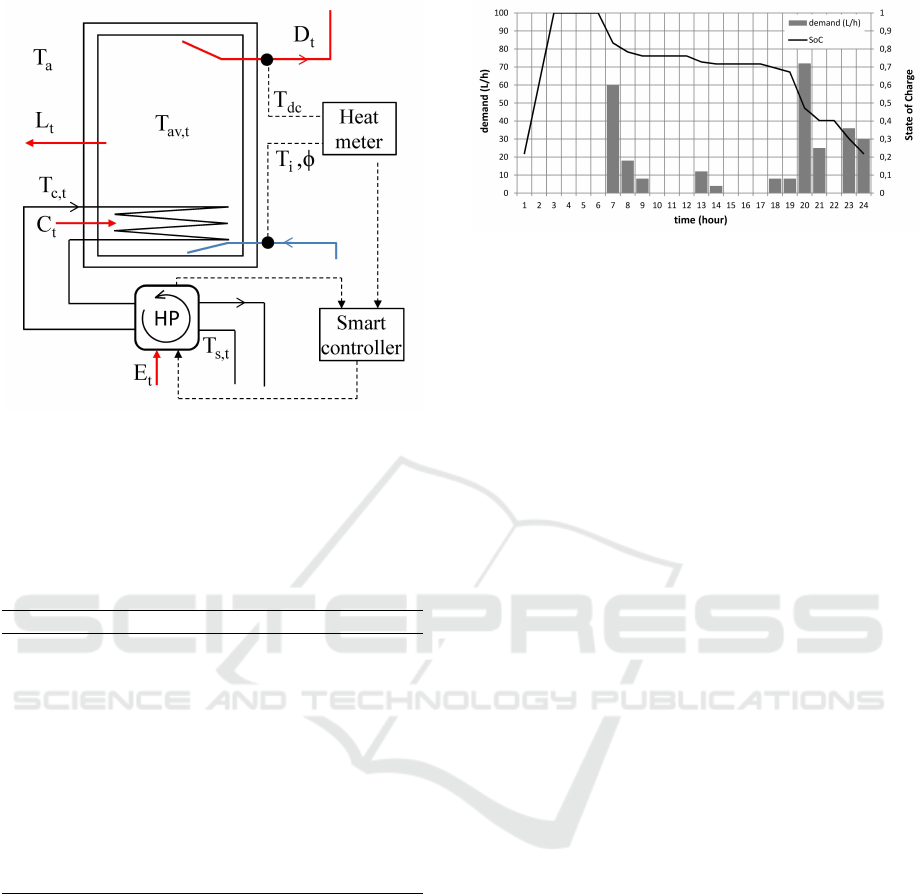
Figure 1: Schematic picture of the thermal storage.

from the top of the storage. A heat pump or solar

collector generates heat which is transferred by a

coil heat exchanger within the bottom region of the

storage tank.

Table 1: Mathematical notations used in Figure 1.

Notation signiﬁcation

charging thermal energy at time t

heat pump electrical energy consumption

loss of thermal energy from the storage

thermal energy demand from the storage

HP heat pump

Φ inlet or outlet water ﬂow

ambient temperature

c,t

charging ﬂow supply temperature

s,t

heat pump source supply temperature

outlet or discharge water temperature

inlet water temperature

av,t

average storage water temperature

The size of the thermal storage is typically 200

liters, sufﬁcient for daily hot water consumption of

households up to 5 persons. The storage may not be

the only hot water system within a house. Hot water

for kitchen use, e.g. to wash dishes, may be supplied

by a separate 10-15 liters electric hot water storage.

The model derived in this section may also be appli-

cable for this type of storage. It is interesting to incor-

porate such storages in a smart energy control system

due to the relatively high power demand, i.e. typi-

cally 2500 W for charging periods ranging from 30

minutes to 2 hours. Figure 1 shows connection of the

storage to a heat meter and smart controller. The heat

meter determines the supplied energy and volume of

hot water. The smart controller determines the actual

Figure 2: Typical daily hot water demand pattern of a

household.

SoC and decides when to start the heat pump (HP) for

charging, based on optimization objectives. We will

discuss this topic further in Section 4.2.

The thermal storage supplies the daily demand for do-

mestic hot water for a single household. The demand

pattern can be learned in time, e.g. as hot water ﬂow

per time interval. For a single house, the uncertainty

on the demand pattern is large if it is evaluated for

small time intervals, but it is smaller if demand is

evaluated for larger time intervals, e.g. as total de-

mand per hour. Figure 2 shows a typical daily demand

pattern of a 4 person household with an annual do-

mestic hot water energy demand of 9 GJ/y (Leeuwen

and Ende, 2016).

The demand pattern is given in liters/hour of 40

◦

The thermal storage has a size of 200 liters and is

charged to 60

◦

C. The SoC of the storage which is

explained in Section 3.2 is charged to 1 early in the

night and drops to nearly 0.21 at the end of the day

due to the discharge of hot water. The daily SoC pat-

tern shows that for the evaluation of the SoC, a resolu-

tion of one hour of the demand prediction is sufﬁcient

in this case.

Another aspect to take into account is the com-

fort of domestic hot water supply. Measures for com-

fort are the water temperature and the availability in

time of warm water. People’s expectations of com-

fort may vary throughout the day. For the control sys-

tem, information about warm water demand and ex-

pected comfort is important in order to decide which

amount of water of a certain temperature should be

at least available within the thermal storage at certain

moments during the day. The predictive model for

charging and discharging the storage should be able

to provide this information.

3.2 Discharging Model and

Experiments

If the storage shown in Figure 1 is ideally stratiﬁed,

the entire volume of hot water with a uniform tem-

SMARTGREENS 2016 - 5th International Conference on Smart Cities and Green ICT Systems

138

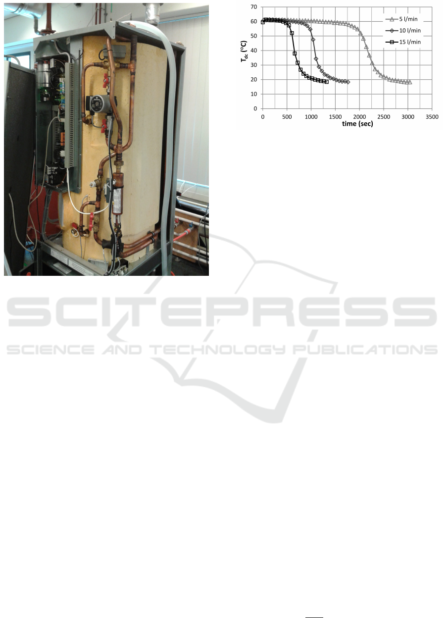
Figure 3: Alpha-Innotec heat pump storage combination

used for testing.

perature moves upwards, perfectly separated from a

growing volume of cold water from the bottom. How-

ever, the incoming cold water ﬂow induces some mix-

ing of cold and hot water. The result is that less water

volume with a high temperature can be drawn from

the tank than in the perfect stratiﬁed case.

To investigate this behavior, experiments are car-

ried out by the energy research lab of Saxion Univer-

sity of Applied Sciences. The experiments involve

charging and discharging cycles for two commer-

cially available, combined heat pump/thermal storage

units. One is a 200 liter combination with a ground

water source heat pump from Alpha-Innotec, refer to

Figure 3. The other is a 50 liter combination with an

air source heat pump from Inventum.

For the hot water storage and for the glycol source

side circuit of the heat pump, the 200 liter combina-

tion is equipped with PT-100 temperature sensors at

the inlets and outlets and ﬂow sensors at the inlets.

The wall socket is equipped with an electric power

sensor. The sensors are connected to a National In-

struments data acquisition system which is connected

to a PC. Labview is used to obtain and log the data.

The 50 liter combination was tested at a user’s site

using a minimum amount of sensors, a PT-100 sen-

sor and a ﬂow sensor on the hot water outlet and an

electric power sensor on the wall socket. A portable

datataker acquisition unit was used which logs the

Figure 4: Outlet water temperature at constant ﬂow rates.

data to memory. On the 50 liter combination, only

a few charge/discharge cycles with constant ﬂow are

carried out to verify the phenomena observed from the

200 liter combination for a combination with a much

smaller storage size.

For the 200 liter combination, in Figure 4 the

discharge temperature (T

) is shown for three con-

stant ﬂow rates. When perfectly stratiﬁed, the storage

should supply hot water with a constant high temper-

ature for 2400, 1200 and 800 seconds for the respec-

tive ﬂow rates of 5, 10 and 15 l/min. However, ﬁgure

4 shows that allready at 2150, 1050 and 650 seconds,

the outlet water temperature has dropped below the

minimum use temperature of 40

◦

C, which demon-

strates the effects of mixing of cold and hot water

within the thermal storage during discharging.

Purpose of the discharging model is to determine:

• the amount of energy supplied from an initial

State of Charge

• the present SoC of the thermal storage

• the amount of useful energy (T ≥ 40

◦

C) that the

storage is still able to supply

Assuming that energy supply from the storage equals

energy demand, the supplied energy in time interval

∆t is calculated with Equation 2.

∆D

= ∆t · φ

· ρ · c

· (T

dc,t

− T

i,t

) (2)

In which ρ the water density and c

the water spe-

ciﬁc heat. In this paper, ρ and c

are assumed constant

although they vary slightly with temperature. When

a heat meter is connected to the thermal storage, the

outlet temperature T

dc,t

, inlet temperature T

i,t

and ﬂow

are registered, which is used to learn the demand in

time. The heat meter calculates the supplied energy

by applying Equation 2. A smart grid algorithm may

use this information to determine the actual SoC of

the thermal storage. The SoC is calculated by Equa-

tion 3.

SoC

max

, 0 ≤ SoC

≤ 1 (3)

A Predictive Model for Smart Control of a Domestic Heat Pump and Thermal Storage

139

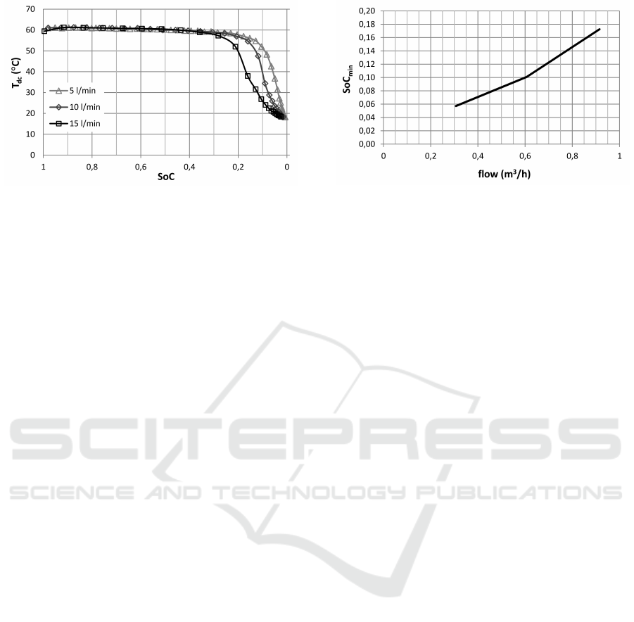
Figure 5: Relation between storage State of Charge and dis-

charge temperature.

The stored energy at time interval t, S

is determined

by Equation 4. S

t−1

is the stored energy at the previ-

ous time interval t −1. The maximum charged energy

is determined by Equation 5, which is worked out

from the ﬁrst law of thermodynamics, relating the re-

quired thermal energy to the change of enthalpy of the

mass of water within the storage (Moran and Shapiro,

2000).

= S

t−1

+ ∆S

(4)

max

= V ·ρ · c

· (T

max

− T

) (5)

In which V the water volume in the storage, T

max

the

maximum, uniform temperature of the storage, i.e.

determined by the storage thermostat settings. The

inlet cold water temperature T

is assumed constant

in this Equation. In practice, a certain volume of the

inlet cold water may warm up to room temperature

conditions due to stand-still heat transfer in the inlet

pipes. The cold water temperature also varies with the

seasons.

The amount of useful energy that can be sup-

plied by the storage is determined by a minimum SoC

value. In ﬁgure 5 the minimum SoC is determined

from the intersection with a supply temperature of

◦

In ﬁgure 6, the minimum SoC is shown as a func-

tion of ﬂow rate. Assuming negligible mixing effects

(or minimum SoC of zero) for a ﬂow rate close to

zero, the minimum SoC appears to increase approxi-

mately linear with ﬂow rate. In practice, ﬂow rates are

not constant but may vary per draw between 5 and 15

l/min. This makes it practicable to use a single value

for the minimum SoC, e.g. the worst case which is

0.18. Together with the calculation of the stored en-

ergy from Equation 4, the minimum SoC value deter-

mines the amount of useful energy that the storage is

still able to supply.

Figure 6: Minimum State of Charge as a function of con-

stant ﬂow rate.

3.3 Charging Model and Experiments

During charging, heat is transferred from the coil at

the bottom to the water in the storage by the principle

of natural convection. From a discharged state, the

water in the storage is cold and during charging the

temperature increases gradually. The heat pump ef-

ﬁciency decreases with increasing water temperature

during the charging process. The heat pump’s refrig-

erant ﬂows through the coil heat exchanger where it

condensates at constant temperature. The coil is usu-

ally made of thin-walled copper, aluminum or stain-

less steel with an approximately negligible conduc-

tion resistance.

Based on supplier heat pump characteristics (Alpha-

Innotec, 2015) and validation measurements, the

charging energy of the heat pump ∆C

appears to be

approximately linear with the source temperature T

s,t

The same characteristics show that the electric energy

∆E is approximately linear with the condenser tem-

perature. Linear equations are developed for C

and

and given in Equation 6.

∆C

= a · T

s,t

+ b

∆E

= c · T

c,t

+ d (6)

In which a, b, c, d are constants which are determined

from supplier data. For the 200 liter heat pump, these

constants are given in Table 2. It is common practice

for domestic heat pumps to measure the condenser

and source temperature for safety reasons, hence the

smart control system should be connected to the heat

pump and obtain this data. The source temperature

may vary in time but this depends on the heat source,

e.g. ambient air varies much more dynamic than

ground water.

Neglecting the coil conductive resistance, the coil

temperature approximately equals the condenser tem-

perature. The heat transfer from the coil to the sur-

rounding water in the storage is given by Equation 7

which is based on Newton’s law of cooling (Moran

SMARTGREENS 2016 - 5th International Conference on Smart Cities and Green ICT Systems

140

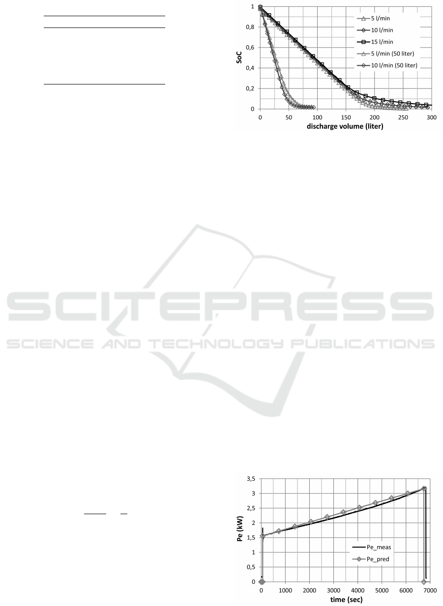
Table 2: Heat pump and coil model parameters.

Parameter Value Unit

a 0.172 kW/K

b -42.2 kW

c 0.04 kW/K

d -10.2 kW

h · A 1.191 kW/K

and Shapiro, 2000).

∆C

= h · A · (T

c,t

− T

w,t

) (7)

In which h the coil heat transfer coefﬁcient, A the coil

outside area and T

w,t

the surrounding water tempera-

ture within the storage. The product h · A is approxi-

mately constant for a complete charging cycle, is ob-

tained from supplier data and given in Table 2. When

the surrounding water temperature is known, equat-

ing ∆C

from Equations 6 and 7 yields the condenser

temperature T

c,t

which determines the electric energy

requirement ∆E

. Hence a suitable prediction of the

water temperature within the thermal storage around

the coil is needed.

When charging from a fully discharged condition, the

water temperature within the storage is approximately

uniform and the left term of Equation 1 is approxi-

mated as:

ρV c

∆T

w,t

(8)

Solving Equation 1 yields the average water tempera-

ture which is then substituted into Equation 7.

However, the storage is usually not discharged beyond

the minimum SoC. In that case, we learn from Figure

4 that a temperature distribution must exist within the

storage, consisting of a layer of hot water at the top

of the storage, a cold layer at the bottom and a mixed

layer in between. During charging, the hot layer at

the top remains in place, while the temperature of the

cold and mixed layer increases gradually. In the fol-

lowing, we develop a suitable approximation based on

the SoC.

In ﬁgure 7 the decrease of the SoC with the total dis-

charged volume from the storage is shown, which in-

dicates a linear decrease down to the minimum SoC

level. For the slope, Equation 9 applies.

∆SoC

∆V

(9)

The model assumes that during charging, the wa-

ter volume in the storage consists of 2 layers: an

upper layer with a uniform hot temperature and a

lower layer with a colder but increasing temperature.

For a given SoC

(SoC

min

≤ SoC

≤ 1), the remain-

ing volume of hot water V

h,t

within the storage can

be calculated with Equation 9 substituting: ∆SoC =

SoC

− SoC

min

, which outputs ∆V which is V

h,t

Figure 7: State of Charge as a function of discharged vol-

ume.

The average temperature T

w,t

in Equation 8, accord-

ing to the model assumption of 2 layers, is the average

temperature of the lower layer of mixed water volume

in the storage, i.e. V −V

h,t

. This temperature is cal-

culated from Equation 10 in which the stored energy

t−1

is known from the state of the previous time in-

terval.

t−1

= ρ·c

·[V

h,t−1

·(T

max

−T

)+(V −V

h,t−1

)·(T

w,t

−T

)]

(10)

Figure 8 shows the measured heat pump electric

power during charging from an empty to a full state of

the storage. During charging, the water temperature

is measured at two locations, at a quarter of the

storage height and at the top. These temperatures

also increase approximately linear and differ only

a few degrees during charging, so we conclude that

during charging from an empty state, the storage

temperature is increased isothermal. Hence, electric

power increases approximately linear with the water

temperature within the storage. It follows that when

the charging process starts from an arbitrary SoC

state, the average water temperature of the water

volume that needs a temperature increase determines

the duration and the amount of electric energy.

Figure 8: Measured electric power during charging.

A Predictive Model for Smart Control of a Domestic Heat Pump and Thermal Storage

141

The total required thermal charging energy is cal-

culated with Equation 12.

tot,t

= (1 − SoC

) · S

max

(11)

SoC

min

≤ SoC

≤ 1 (12)

The duration of the charging process τ

is calculated

with Equation 13

tot,t

∆C

(13)

In which ∆C

is calculated with Equation 6. The elec-

tric power consumption proﬁle P

e,t

∗

of a future charg-

ing cycle with discrete time t

∗

in the future, from a

given SoC

to fully charged conditions, is predicted as

a linear function in time, Equation 14 which starts at a

value P

e,t

∗

and ends with P

e,t

∗

+τ

. These values are cal-

culated with ∆E

, Equation 6. t

∗

is some time in the

future when charging is initiated, which is a control

variable for the smart control system.

e,t

∗

= P

e,t

∗

e,t

∗

+τ

− P

e,t

∗

·t

∗

0 ≤ t

∗

≤ τ (14)

The electric energy consumption of the future charg-

ing cycle is calculated with Equation 15, which is the

integral of Equation 14.

tot,τ

· (P

e,t

∗

+ P

e,t

∗

+τ

) (15)

With the parameters given in Table 2 the values shown

in Table 3 are calculated for the charging cycle of Fig-

ure 8. In this ﬁgure, the resulting prediction proﬁle is

also shown for comparison and this demonstrates the

excellent accuracy of the approach.

Table 3: Comparison between prediction and measurements

of electric energy consumption.

Result Measured Predicted Unit

τ 6763 6677 sec

e,t

∗

1.45 1.56 kW

e,t

∗

+τ

3.21 3.16 kW

tot,τ

15564 15759 kJ

3.4 Energy Loss

When the storage is charged and discharged daily, en-

ergy losses from the storage to the surrounding air are

insigniﬁcant due to good insulation of modern ther-

mal storage tanks. However, when the storage is not

discharged for many days and placed in a relatively

cold environment, losses may be more signiﬁcant.

The heat loss ∆L

is calculated by the general heat

transfer relation (Moran and Shapiro, 2000), Equation

16.

∆L

= UA · (T

av,t

− T

a,t

) (16)

In which UA the storage heat loss coefﬁcient, T

av,t

the

average storage temperature and T

a,t

the ambient air

temperature which may be assumed constant in time,

depending on the situation. Assuming constant wa-

ter density and speciﬁc heat, T

av,t

is calculated with

Equation 17.

V · T

av,t

= V

h,t

· T

max

+ (V −V

h,t

) · T

w,t

(17)

3.5 Validation Experiments

Validation of the model is performed by discharging

the storage with constant ﬂow φ starting at SoC=1 to

SoC

end

, followed by charging to SoC=1. Values for φ

and SoC

end

are given in Table 4.

Table 4: Validation experiment settings.

Experiment φ (l/min) SoC

end

1 5 0.6

2 10 0.6

3 15 0.6

4 10 0.4

5 10 0.2

During discharging, ﬂow and temperature are

measured of the inlet and outlet water. During charg-

ing, electric energy consumption is measured. The

model prediction algorithm involves:

1. determine actual SoC from measured ﬂow and

temperatures, Equations 1, 2 and 3

2. determine required charging energy C

tot

, Equation

3. calculate duration τ of future charging cycle,

Equation 13

4. calculate average water temperature of cold and

mixed water layer in thermal storage, Equation 10

and condenser temperature at the beginning and

end of a future charging cycle, Equation 7

5. determine minimum and maximum electric power

of charging cycle P

e,t

∗

and P

e,t

∗

+τ

, Equation 6

6. determine total electric energy consumption dur-

ing charging cycle E

tot

, Equation 15

The validation compares model predictions of dura-

tion τ, minimum and maximum electric power P

e,t

∗

and P

e,t

∗

+τ

and total electric energy consumption E

tot

which characterize the future charging cycle with the

measured charging cycle.

SMARTGREENS 2016 - 5th International Conference on Smart Cities and Green ICT Systems

142

Table 5: Validation results.

Experiment τ

meas

% error P

e,t

∗

e,t

∗

+τ

MAX % error T

w, pred

tot,meas

% error

(sec) τ (kW) (kW) ∆P

◦

C (kJ) E

tot

1 2911 -7.2 2.17 3.20 6.2 31.2 14872 0.3

2 2637 2.5 2.10 3.22 5.6 29.9 14465 3.1

3 2973 -9.1 2.16 3.22 5.4 31.6 15018 -0.7

4 4050 -1.6 1.86 3.22 8.7 27.6 22352 0.1

5 5229 1.1 1.85 3.23 5.2 25.4 29662 0.1

4 RESULTS AND DISCUSSION

4.1 Validation Results

The validation results are shown in Table 5. The mea-

sured duration τ

meas

, measured minimum and maxi-

mum electric power consumption P

e,t

∗

and P

e,t

∗

+τ

and

measured total electric energy consumption E

tot,meas

are listed for each experiment. The error of the predic-

tions is given as a percentage of the measured values.

For the predictions, the average water temperature of

the cold and mixed water layer T

w, pred

calculated from

Equation 10 is shown, from which the electric power

at the start of the charging cycle is predicted.

For the future charging cycle, accurate prediction

of the total electric consumption and duration are the

most important aspects for smart energy control pur-

poses. Table 5 indicates an excellent prediction accu-

racy of the total electric consumption, while in most

cases the percentage error is smaller than 1%. Al-

though the prediction of duration seems less accurate

in some cases, the maximum error of 9.1% is only a

difference of 4.5 minutes. Smart energy control algo-

rithms usually evaluate predictions in time intervals

of 15 minutes, hence this maximum error is accept-

able.

For the prediction of the energy consumption pro-

ﬁle, the maximum error (8.7%) is 280 W, which ap-

pears at the end of the charging cycle. This error is

mainly due to differences in the same order of mag-

nitude between supplier data of electric power con-

sumption which is used for the model and actual mea-

surements of electric power consumption. We veriﬁed

that if the constants c, d in Equation 6 are based partly

on supplier data and partly on the measured power

consumption at the end of charging, the prediction

proﬁle is more accurate. This information could be

made available to the control system by a connected

smart electricity meter.

It also has to be taken into account that the errors

are in the same order of magnitude as the propagated

measurement errors of the used sensors. Therefore

we conclude that the predictive model is very well ca-

pable to accurately predict the duration, power con-

sumption and power consumption proﬁle for future

charging cycles of the thermal storage.

4.2 Case Application

Application of the model is investigated with a case

for increased self-consumption of domestic solar PV

electricity. Figure 9 shows a reference proﬁle of a

day in the spring season. The proﬁle is constructed

speciﬁcally as a case for this paper and based on

measured data on electricity consumption of a four

person household and weather data. The ﬁgure

shows electric power consumption and solar PV

generation without smart control. The yearly sum

of daily base loads totals 2600 kWh/y and includes

electricity consumption of lights, dishwasher, wash-

ing machine, washing dryer, television, computer and

small electronic devices. The base load is considered

non-ﬂexible in this case. The heat pump which

charges the thermal storage is a ﬂexible device which

can be controlled by a smart controller, as indicated

in Figure 1. The reference case shows that solar PV

energy generation during the day is mostly exported

to the grid, while the occupants are mostly out of

the house during the day and come home around

17.00 hours. Financially, this may be unfavorable,

depending on the feed-in tariff. Besides this, charging

energy of the heat pump and SoC of the thermal

storage are shown. The total proﬁle illustrates the

load on the power grid, ranging from a feed-in peak

of -1380 Wh during the day to a demand peak of

3020 Wh during the night.

Figure 9: Reference electricity consumption and solar PV

generation proﬁle.

A Predictive Model for Smart Control of a Domestic Heat Pump and Thermal Storage

143

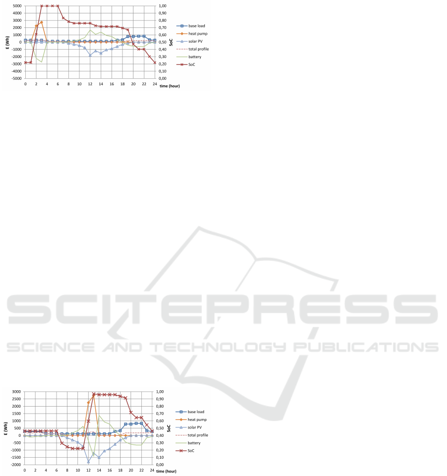
Figure 10: Variant 1: electricity proﬁle with optimized elec-

tric battery storage.

Figure 10 shows results for variant 1 which in-

cludes an electric battery which is able to charge when

there is a surplus of electricity generation and to dis-

charge when there is insufﬁcient generation. The

hourly amounts of charged and discharged energy are

determined by an optimization algorithm which min-

imizes peaks of the total proﬁle. The optimization

algorithm used is explained in detail in (Fink et al.,

2015). The required battery capacity for this proﬁle is

calculated at 7.34 kWh. The electricity consumption

peak is reduced to 293 Wh during the night.

Figure 11 shows results for variant 2 which in-

cludes an electric battery and smart control of the heat

pump. Besides minimizing peaks of the total proﬁle,

the control algorithm minimizes capacity of the elec-

tric battery. The thermal storage and heat pump charg-

ing model developed in this paper are included in the

control algorithm to predict SoC and electricity con-

sumption. As result, the required battery capacity is

decreased to 4.58 kWh and the electricity consump-

tion peak is now 256 Wh which occurs during day-

time hours.

Figure 11: Variant 2: electricity proﬁle with optimized heat

pump control and electric battery storage.

The results of variant 2 have several positive effects:

• decreased battery capacity and lower investments

compared to variant 1

• lower electricity peak values compared to variant

• shift of electricity shortage towards daytime

hours, allowing more local consumption of other

renewable energy generation in the district

Main purpose of the case study is to show the signiﬁ-

cance of model prediction of energy for charging the

thermal storage. A more elaborate case study involv-

ing different households, more days throughout the

year and comparisons with thermostat thermal stor-

age control is required to study the effects of smart

control more thoroughly.

5 CONCLUSIONS

In this paper a predictive model is developed for a do-

mestic hot water thermal storage which is charged by

a heat pump. The model is derived from heat bal-

ance equations combined with insights from experi-

mental data. The model involves a set of relatively

simple algebraic equations which are easy to evalu-

ate by smart energy control algorithms without itera-

tions. Required inputs are: recordings of measured in-

let and outlet water temperature and water ﬂow, which

can be performed by low cost heat meters in practice.

Outputs of the predictive model are: duration, elec-

tric consumption proﬁle and total electric energy con-

sumption of a future charging cycle by the heat pump

from the present state of charge to fully charged con-

ditions.

Accuracy of the model is validated by comparing

results of model predictions with experimental ﬁnd-

ings. The percentage error on the predicted duration

of the charging cycle is between 1% and 9%, on the

electric power consumption between 5% and 9% and

on the total electrical energy consumption lower than

3%.

Hence the model can be applied for similar do-

mestic hot water storage conﬁgurations, although the

relations introduced which describe heat pump elec-

tric power consumption, may be different for differ-

ent types of heat pumps and different heat pump con-

trol systems. Changing these relations is however a

relatively simple task which involves analysis of the

heat pump characteristics, either from supplier data

or by executing a few discharging/charging cycle ex-

periments.

Application of the model is investigated with a

case of increased self consumption. The developed

predictive model is relatively easy to implement into

an optimization control algorithm which minimizes

peak electricity consumption of a household and elec-

tric battery capacity. The results for this type of con-

trol show decreased battery capacity, lower electricity

peak values and a shift of hours of electricity shortage

from nighttime to daytime hours, which is favorable

for local consumption of renewable energy generation

in a district. Future work is aimed at integration of

SMARTGREENS 2016 - 5th International Conference on Smart Cities and Green ICT Systems

144

the model into the Triana smart grid simulator which

is used for simulation studies and as base for embed-

ded smart control systems. We will also investigate

suitable methods for domestic hot water demand pre-

diction as part of smart energy control of the thermal

storage and heat pump.

ACKNOWLEDGMENT

The authors would like to thank the Dutch national

program TKI-Switch2SmartGrids for supporting the

project Meppelenergy and the STW organization for

supporting the project I-Care 11854. We also thank

Nathan imports for making an Alpha-Innotec heat

pump/storage combination available and GEAS for

letting us test an Inventum heat pump/storage com-

bination.

REFERENCES

Alpha-Innotec (2015). Brine/water heat pumps, WZS series

- operating manual. UK830501/200520.

Baeten, B., Rogiers, F., Patteeuw, D., and Helsen, L. (2015).

Comparison of optimal control formulations for strat-

iﬁed sensible thermal energy storage in space heating

applications. In The 13th International Conference on

Energy Storage.

De Ridder, F. and Coomans, M. (2014). Grey-box

model and identiﬁcation procedure for domestic ther-

mal storage vessels. Applied Thermal Engineering,

67(1):147–158.

Fan, J. and Furbo, S. (2012). Thermal stratiﬁcation in a

hot water tank established by heat loss from the tank.

Solar Energy, 86(11):3460–3469.

Fink, J., Leeuwen, R. v., Hurink, J., and Smit, G. (2015).

Linear programming control of a group of heat pumps.

Journal Energy, Sustainability and Society, (2015)

5:33.

Halvgaard, R., Bacher, P., Perers, B., Andersen, E., Furbo,

S., Jørgensen, J. B., Poulsen, N. K., and Madsen, H.

(2012). Model predictive control for a smart solar tank

based on weather and consumption forecasts. Energy

Procedia, 30:270–278.

Han, Y., Wang, R., and Dai, Y. (2009). Thermal stratiﬁca-

tion within the water tank. Renewable and Sustainable

Energy Reviews, 13(5):1014–1026.

Henze, G. P., Felsmann, C., and Knabe, G. (2004). Evalu-

ation of optimal control for active and passive build-

ing thermal storage. International Journal of Thermal

Sciences, 43(2):173–183.

Kleinbach, E. M., Beckman, W., and Klein, S. (1993). Per-

formance study of one-dimensional models for strati-

ﬁed thermal storage tanks. Solar energy, 50(2):155–

166.

Kriett, P. O. and Salani, M. (2012). Optimal control of a

residential microgrid. Energy, 42(1):321–330.

Leeuwen, R. v. and Ende, J. v. t. (2016). Domestic thermal

energy consumption patterns - comparing model pre-

dictions with data. Technical Report report 20160630,

Saxion University of Applied Sciences.

Leeuwen, R. v., Fink, J., and Smit, G. (2015). Central model

predictive control of a group of domestic heat pumps,

case study for a small district. In Proceedings Smart-

greens 2015, 4rd International Conference on Smart

Cities and Green ICT Systems, Lissabon, Portugal,

20-22 May, 2015, pages 136–147.

Moran, M. and Shapiro, H. (2000). Fundamentals of Engi-

neering Thermodynamics. Wiley, 4 edition.

Nykamp, S. (2013). Integrating renewables in distribution

grids - storage, regulation and the interaction of dif-

ferent stakeholders in future grids. PhD thesis, Uni-

versity of Twente.

Oliveski, R. D. C., Krenzinger, A., and Vielmo, H. A.

(2003). Comparison between models for the sim-

ulation of hot water storage tanks. Solar Energy,

75(2):121–134.

Rosen, M. A. (2001). The exergy of stratiﬁed thermal en-

ergy storages. Solar energy, 71(3):173–185.

A Predictive Model for Smart Control of a Domestic Heat Pump and Thermal Storage

145