Land Cover Clustering based on Improved Dictionary Learning Method

from Modis Data

Mariem Zaouali, Sonia Bouzidi and Ezzeddine Zagrouba

RIADI Laboratory, Research Team on Intelligent Systems in Image and Artiﬁcial Vision, ISI,

University of Tunis El Manar, Tunis, Tunisia

Keywords:

k-Means Clustering Algorithm, Discriminative Temporal Behavior, Dictionary Learning, Coarse Spatial

Resolution Images, Remote Sensing, Sparse Representation.

Abstract:

An approach based on k-means clustering algorithm combined with the concept of sparse representation is

proposed in this paper. We intend to discriminate, each vegetation type, by its temporal behavior. Our method

is composed of two main parts : The ﬁrst part consists of designing the dictionary that we are going to use.

For this reason, we propose a modiﬁcation of the k-svd algorithm by switching the use of OMP algorithm

by the SunSAL algorithm. Then we carry on an unsupervised clustering process using k-means algorithm on

sparse vectors. As a result, we found that SunSAL algorithm outperforms the OMP algorithm and we succeed

to elaborate discriminative temporal behaviors of the vegetation in our region of study. As perspectives, our

approach could be considered as an attempt to overcome the shortage of high spatial resolution data since we

are relying only on coarse remote sensing images like MODIS to monitor Land Cover dynamics.

1 INTRODUCTION

Over the past decades, remote sensing measurements

have played a key role in analyzing climate changes

and dynamics of ecosystem, in order to protect the

Earth surface from environmental disasters. Nowa-

days, thanks to the development of aerospace tech-

nologies, a great number of satellite sensors has been

launched, which has increased incredibly the amount

of available data. The use of multitemporal coarse

resolution satellite imagery has shown potentials but

requires a considerable amount of data, especially

ground truth, to monitor land cover change (Zhan

et al., 2002; Morton et al., 2005). Thus, unsuper-

vised methods give a more attractive solution to that.

In this work, we explore a coarse spatial resolution

data but highly frequent in time. We estimate that

the temporal features is interesting to model the land

cover and could improve vegetation cover classiﬁca-

tion (Jia et al., 2013). Indeed, time series vegetation

index (eg. NDVI or EVI) are approved to well de-

scribe vegetation growth as well as revealing the veg-

etation type information since it represents the phe-

nology cycle (Brown et al., 2013). Whereas, the main

issue comes to how surpass dimensionality of time se-

ries data and limited availability of labeled samples

to improve land cover classiﬁcation accuracy. In a

recent work (Yang et al., 2014), an approach is pro-

posed based on NDVI, PCA and ISODATA cluster-

ing algorithm (which groups pixels with similar spa-

tial and spectral characteristics into classes (Moham-

mady et al., 2015)). However, in practical application,

the quality of this classiﬁcation is often not enough

(Guha and Ward, 2012). Recently, sparse model-

ing has proven fruitful application in various ﬁelds

such as signal, image, compression and others (Lim

et al., 2012; Mahmoudi and Sapiro, 2012; Wright

et al., 2009). It also provides a useful tool for ma-

chine learning. In fact, sparse representation can clas-

sify any samples based on the concept that it is a lin-

ear combination of labeled prototype samples (Chen

and Donoho, 1994). In this work, we tried to exploit

sparse representation paradigm since it is a tool for

dimensionality reduction, in order to conduct unsu-

pervised clustering. The idea is to ﬁnd a dictionary

that can well approximate NDVI temporal behavior

without the requirement of labeled samples. The ﬁ-

nal result is a discriminant temporal behavior of each

land cover and a labeled data. This paper is organized

as follows: Section II presents Related concepts, Sec-

tion III describes the proposed approach, Section IV

presents the Study area, Section V describes experi-

mental protocol and results. Finally the last Section is

the conclusion.

Zaouali, M., Bouzidi, S. and Zagrouba, E.

Land Cover Clustering based on Improved Dictionary Learning Method from Modis Data.

DOI: 10.5220/0005851006970704

In Proceedings of the 11th Joint Conference on Computer Vision, Imaging and Computer Graphics Theory and Applications (VISIGRAPP 2016) - Volume 4: VISAPP, pages 697-704

ISBN: 978-989-758-175-5

697

2 RELATED CONCEPTS

Sparse representation helps having compact represen-

tation of images by using a reduced set of coefﬁcients

from a basis of elements, i.e dictionary, which is a

matrix whose columns d

are called atoms. This tech-

nique has been applied in various ﬁelds including re-

mote sensing. In our case, we want to exploit sparse

representation in order to improve land cover classiﬁ-

cation and then use it for changes detection. We aim

to discriminate classes by their temporal behavior in

order to make detecting changes easier. This would

be an attempt to deal with limited availability of la-

beled samples. Our approach is based on considering

temporal patches as dictionary atoms This means that

we track the temporal behavior of a pixel through the

time series images. In this section, we present the def-

inition of sparse representation and its classiﬁer logic.

2.1 Sparse Representation

Let the dictionary D ∈ R

n×p

be a base containing p

atoms, , each one composed of n rows, with n < p.

This dictionary contains a set of temporal behaviors

chosen randomly from the study area. For a given sig-

nal Y, it is demanded to ﬁnd a sparse vector X, having

only few non zeros coefﬁcients, combining linearly

the atoms of dictionary D. This problem could be pre-

sented in equation 1:

argminkX k

sub ject to kY − DXk

≤ δ (1)

with Y is the signal to represent via X from D and δ

is the level of sparsity. Due to the presence of pos-

sible modeling error and noise, equation (1) is often

replaced by

argminkX k

sub ject to kY − DXk

≤ δ (2)

where kX k

∑

i=1

|. This is due to the difﬁculty

to resolve l

norm, which is considered as NP-hard

problem. In fact, several algorithms have been pro-

posed to solve equation (1) such as Basis pursuit BP

(Chen and Donoho, 1994), Orthogonal Matching Pur-

suit OMP (Tropp et al., 2007) and Sparse UNmixing

by variable Splitting and Augmented Lagrangian Sun-

SAL (Bioucas-Dias and Figueiredo, 2010). BP re-

places the l

norm with l

norm as mentioned in equa-

tion (2). However, OMP proposes a greed strategy. In

the ﬁrst iteration, OMP takes the test sample Y as an

initial residual, then, through each iteration, OMP has

to recognize the atom that could best approximate the

residual. Using the selected atoms, OMP re-estimates

X. This algorithm will stop once if one of the fol-

lowing conditions are met: Approximation error is

less than a certain threshold or a predeﬁned number

of atoms have been selected. However SunSAL pro-

poses another approach. It is based on the fact that

the equation (1) is equivalent to the following uncon-

strained optimization problem:

min

ky − Dxk

+ λkxk

(3)

where λ is a Lagrangian multiplier. SunSAL provides

an efﬁcient solution form l

− l

norm problem. It is

considered more efﬁcient and less complex with equal

accurate solution as an alternate of LASSO-(least ab-

solute shrinkage and selection operator)(Xue et al.,

2015). In this work, we deal with OMP and SunSAL

and compare their performance in designing dictio-

nary. In next section, we describe how, with the help

of dictionary and sparse representation, we can clas-

sify training samples.

2.2 Sparse Representation based

Classiﬁer

Sparse representation relies on the idea that any signal

is a linear combination of atoms belonging to a class.

That is mean that any signal representing a class C

could be sparsely composed by remarkable coefﬁcient

of class C

while for the other class, are barely zeros.

Indeed, for a set of k objects of classes : v

i,1

, ...v

i,k

with v

i, j

is the j

sample of the i

class, let consider

= [v

i,1

, ...v

i,k

] as the matrix representing the i

. Let

D= [D

, D

, ...D

] be a dictionary. The resolution of

Y = DX with X = [0, ....0, x

i,1

, x

i,2

, ..., x

i, j

, 0.....0]

the sparse vector, gives us the label of the sample Y .

In fact X would have only few non zero coefﬁcients

which refer to the class of Y . Thanks to the residual

base criterion formula :

class(y

) = arg min

j∈1...c

kY − DXk

(4)

where class(y

) is the class label affected to y, we can

measure the accuracy of the classiﬁcation result. In

our case, we cannot determine the label of samples y

because the dictionary atoms’ are anonymous. They

just were extracted from the study region without any

further information pertaining to its type. The pro-

posed solution to this point, is described in the next

section.

3 PROPOSED APPROACH

In this work, we try to classify vegetation based on its

discriminant behavior using NDVI (Normalized Dif-

ferential Vegetation Index) proﬁles. This index is de-

ﬁned as the difference between the visible (red) and

RGB-SpectralImaging 2016 - Special Session on RBG and Spectral Imaging for Civil/Survey Engineering, Cultural, Environmental,

Industrial Applications

698

near-infrared (nir) bands, over their sum. It is directly

related to the amount of photo synthetically-active ra-

diation intercepted by the vegetation canopy, and thus

it is widely used for differentiating areas that contain

healthy vegetation. We aim, in this paper, to charac-

terize the phenology of vegetation through its NDVI

proﬁles. To reach this goal, we propose, an approach

based on sparse representation and dictionary learn-

ing. In literature, dictionary could be pre-designed or

resulting from training process. The choice of which

dictionary to use, is established according to the appli-

cation context. In our work, we have chosen to con-

Sequence of

images - MODIS

Dictionary learning

NDVI Temporal

Behavior of pixels

K-means performed on sparse vectors

Number of clusters fixed by Silhouette method

Mean of Temporal Profiles of each cluster

dates

NDVI

Extract temporal

patches to plot

NDVI Temporal

behavior

Dictionary initialization : atoms are NDVI Temporal Behavior

dates

Figure 1: Proposed approach.

duct a dictionary learning process in order to ﬁt the

data and to characterize it only through its temporal

behavior not through its spatial characteristics. Thus,

in our case, we edit the K-SVD algorithm (Aharon

et al., 2006) to do this learning: The ﬁrst step is the

dictionary initialization, we choose randomly samples

from the study area which would be used as the atoms

of dictionary. The design of the dictionary consists of

two steps:

• Sparse coding where we determine the dictionary

atoms’ ﬁtting given samples

• Dictionary update where we edit the atoms of

dictionary in order to minimize approximation er-

ror.

In this paper, we propose an amelioration of the K-

SVD algorithm consisting of substituting the OMP

algorithm in sparse coding step, by the SunSAL algo-

rithm. Thus, Algorithm 1 presents the usual K-SVD

and Algorithm 2 presents its modiﬁcation. We used

them in our experimentation in order to compare their

performance.

Since we don’t have labeled data, we cannot deter-

mine the classes’ labels of the samples using residual-

based criterion of formula (4) described in previous

section. Thus, we perform k-means algorithm to re-

group signals having similar linear atoms combina-

tion into clusters. We vary the cluster’s number in

Algorithm 1: Dictionary Design - K-SVD.

Data: Test Samples Y, initial dictionary D

Result: The learned dictionary D’

• Sparse Coding solving

argminkxk

sub ject to ky − Dxk

≤ δ (5)

• Dictionary Update minimmize E : E = Y -

∑

using SVD, repeat until error E remains

unchanged, where d

is the jth atom of the

dictionary and x

is the ith element of a

column of the sparse vector x.

Algorithm 2: Dictionary Design - K-SVD modiﬁed.

Data: Test Samples Y, initial dictionary D

Result: The learned dictionary D”

• Sparse Coding solving

min

ky − Dxk

+ λkxk

(6)

• Dictionary Update minimmize E : E = Y -

∑

using SVD, repeat until error E remains

unchanged, where d

is the jth atom of the

dictionary and x

is the ith element of a

column of the sparse vector x.

order to ﬁnd which of them gives the best silhouette

values(Rousseeuw, 1987). The silhouette value can

be calculated for each point and represents a measure

of similarity of a given point to the other points in

its own cluster (intra cluster distance), compared to

points belonging to other clusters (inter cluster dis-

tance). For the i

point, Si, is deﬁned as:

Si =

− a

max(a

, b

)

(7)

where a

is the average distance from the i

point to

the other points in the same cluster as i, and b

the minimum average distance from the i

point to

points in a different cluster, minimized over clusters.

Si value varies from -1 to 1. High values indicate that

a given point ﬁts its own cluster and weakly matched

to others. If we have many negative Silhouette values,

this means that the clustering process has whether de-

composed the samples in too many or few clusters.

Whereas, if we get many positive Silhouette values,

this means that the result of the clustering process is

appropriate.

The following Algorithm 3 exhibits the unsuper-

vised clustering process :

After running this algorithm, we compute the dis-

Land Cover Clustering based on Improved Dictionary Learning Method from Modis Data

699

Algorithm 3: Unsupervised Clustering.

Data: Time series images T, learned

dictionaries D’ and D” obtained from the

previous algorithms

Result: Clusters of training samples

• Step 1: Extract randomly temporal samples from T

and reconstruct it using OMP or

SunSAL over respectively D’ and D” dictionaries

• Step 2: Calculate the Silhouette value of the sparse

vectors resulting from the previous step, in order to

determine the number of clusters

• Step 3: K means clustering algorithm on sparse

vectors using the number of clusters found in step 2

criminant temporal behavior of each cluster which is

the mean of all intra-cluster temporal behavior. This

procedure helps us to reduce dimensionality since we

conduct clustering process on sparse vectors instead

of large signals. The Figure 1 exhibits an overview

of the proposed approach.

4 STUDY AREA AND DATA

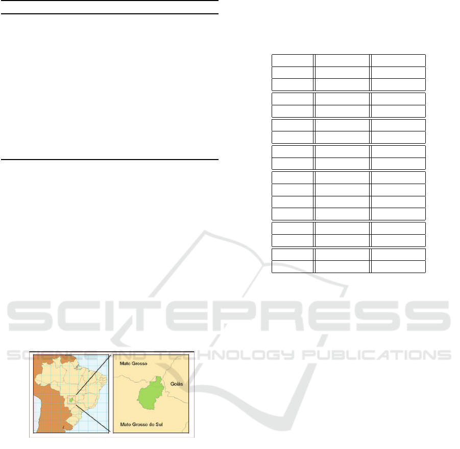
The study area corresponds to Taquari basin, located

almost entirely in the state of Mato Grosso do Sul in

the Center-West of Brazil - Figure 2.

Figure 2: The state of Mato Grosso do Sul in the Center-

West of Brazil.

We have a time-series data from MODIS-Terra

satellite, ”Vegetation Indices 16 days L3 Global 250

m” product which has two indices and ten other chan-

nels for each image: the NDVI and EVI (Enhanced

Vegetation Index). We have used only the NDVI

channel thanks to its relevance (Jonathan et al., 2005).

The used time series contains 26 acquisitions, span-

ning a period from August 2000 to July 2001 which

considered as signiﬁcant to track vegetation evolution

(complete phenology cycle). For the validation phase,

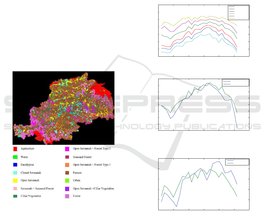
we have a classiﬁcation image at MODIS scale - Fig-

ure 3, elaborated from a Landsat image and expert

validation. We have to emphasize that having a well

documented study region is considered challenging.

Table 1: Silhouette values resulted from the variation of

cluster number which are the input of kmeans algorithm.

The data to be clustered are sparse vectors resulted from the

two algorithms of Dictionary Learning: Algo1(K-SVD) and

Algo2(K-SVD modiﬁed).

nb clus DL:Algo1 DL:Algo2

1 NaN NaN

2 0.5809 0.8489

3 0.3581 0.7364

4 0.2247 0.7331

5 0.1802 0.6881

6 0.1813 0.7059

7 0.1611 0.6208

8 0.1949 0.6792

9 0.1361 0.6287

10 0.1768 0.6589

11 0.1125 0.6529

12 0.1737 0.6694

13 0.1142 0.6623

14 0.1065 0.5945

15 0.0882 0.6521

20 0.1042 0.5400

5 EXPERIMENTAL PROTOCOL

AND RESULTS

In this section, we evaluate the proposed approach by

using MODIS time series data which contain 26 ac-

quisitions. We focussed on the following parameters

because they have a signiﬁcant impact on the result:

• Since the temporal proﬁles of the pixels were

noisy which could probably affect the ﬁnal clas-

siﬁcation result, we proceeded to ﬁlter them by

applying discrete wavelet transform (Daubechies

functions)

• Dictionary: In order to consider all the possible

types of vegetation, when creating our dictionary,

we chose atoms from different regions that cover

most of the studied area

• For the level of sparsity δ mentioned in equation

(2), we varied δ empirically, until reaching a min-

imum value of MSE. This value was ﬁxed to δ =

This experiment is conducted on two dictionaries.

The size of each one of them is 26 × 4868 where 26

is the number of dates, 4868 is the number of atoms.

They are trained using both K-SVD and K-SVD mod-

iﬁed algorithm as mentioned in Algorithm 1 and 2 re-

spectively. Next, we run kmeans using different num-

ber of clusters : 1,2,3..to 20. To ﬁnd out which is the

RGB-SpectralImaging 2016 - Special Session on RBG and Spectral Imaging for Civil/Survey Engineering, Cultural, Environmental,

Industrial Applications

700

appropriate number, we calculate the silhouette value

of each resulted cluster. This value indicates whether

the cluster needs to be further divided or not. The

results are illustrated in Table 1 showing silhouette

values’ variation according to the number of clusters.

The lines correspond to the number of clusters used

in kmeans, and columns correspond to the algorithm

used to train the dictionary.

According to Table 1, the use of SunSAL as clas-

siﬁer, has led to better silhouette values. In fact, all

the SunSAL’s silhouette values are near to 1 which

means we have a good segregation ratio. Here Sun-

SAL suggests that the data could be divided in k = 6

clusters while OMP suggests that k = 8. Thanks to

this table, we discard the classiﬁer OMP because of

its very low silhouette values and we keep SunSAL

classiﬁer since it grants better results. So with k = 6,

we obtain 6 clusters where the mean proﬁles are rep-

resented in Figure 4. To evaluate our experimental

result, we use a ground truth of the studied region de-

scribed in (Jonathan et al., 2005) (Figure 3).

Figure 3: Reference Classes (Jonathan et al., 2005).

Our aim is to match the clusters found by kmeans to

the classes of ground truth in order to identify the

land cover types. So we calculate the Mean Square

Error (MSE) between the estimated temporal behav-

iors and the reference classes. The Table 2 presents

in columns the ground truth classes and in lines the

label of clusters belonging to kmeans algorithm re-

sult. This table helps us ﬁnding the land cover types

corresponding to clusters. For example, according to

Table 2, cluster 2 corresponds to Ciliar Vegetation

and Open Savannah, while cluster 6 corresponds to

Forest. This is conﬁrmed in Figure 5 where we su-

perpose the mean proﬁle in cluster 2 with the mean of

Ciliar Vegetation and Open Savannah. We have done

the same thing to cluster 6 by superposing it with the

Forest proﬁle of ground truth in Figure 6.

Whereas cluster 5 is confused with several classes

: Closed Savannah, Seasonal Forest and Open Savan-

nah + Forest Type 1. This could be explained by the

fact that those 3 classes have close temporal proﬁles

and thus we could regroup all of them in a one single

proﬁle.

0 5 10 15 20 25 30

0.4

0.5

0.6

0.7

0.8

0.9

Dates

NDVI values

X1 = Cluster 1

X2 = Cluster 2

X3 = Cluster 3

X4 = Cluster 4

X5 = Cluster 5

X6 = Cluster 6

Figure 4: Mean proﬁles of the 6 found clusters.

0 5 10 15 20 25 30

0.4

0.45

0.5

0.55

0.6

0.65

0.7

0.75

0.8

Dates

NDVI values

X1 = Class 2

X2 = Cluster 2

Figure 5: A: Superposition of Cluster 2 mean proﬁle with

the mean proﬁle of Ciliar Vegetation and Open Savannah.

0 5 10 15 20 25 30

0.65

0.7

0.75

0.8

0.85

0.9

Dates

NDVI values

X1 = Class 6

X2 = Cluster 6

Figure 6: Superposition of Cluster 6 mean proﬁle with the

Forest proﬁle.

So, thanks to our approach, we have found clusters

that gather more than one ground truth classes. Table

3 shows matching result of our clusters with ground

truth classes. By this way, based on information in

Table 3, we can generate labeled dictionary by deter-

mining to which class, each atom belongs.

We succeed to identify the majority of classes, but

we estimate that some of them are not well recognized

Land Cover Clustering based on Improved Dictionary Learning Method from Modis Data

701

Table 2: Table 2 of MSE values of Sunsal classiﬁer, where A=Argriculture, B=Water,C=Eucalyptus,D=Open Savannah,

E=Closed Savannah, F=Forest, G=Seasonal Forest, H=Ciliar Vegetation I= Open Savanah+ciliar vegetation, J=Open Sa-

vanah+Forest type 1, K= Open Savanah+Forest type 2, L= Savannah+ Seasonal Forest, M=Pasture, N=Urban.

A B C D E F

1 0,013702123 0,014358648 0,00394132 0,014724775 0,045046558 0,072690414

2 0,043921584 0,022896723 0,031124566 0,002306937 0,007234252 0,019553144

3 0,020523329 0,016096906 0,010706222 0,007059779 0,026975737 0,049272183

4 0,01338676 0,017668488 0,002655275 0,029399763 0,072473686 0,105373549

5 0,076233369 0,042593683 0,060901952 0,009707884 0,001062428 0,005719512

6 0,110176038 0,065631921 0,09301972 0,023370714 0,004278307 0,001799481

G H I J K L

1 0,056415746 0,011683206 0,006053524 0,052763398 0,005628253 0,003442471

2 0,01302728 0,001776301 0,006218013 0,010195047 0,012103119 0,008181732

3 0,037179256 0,00419623 0,002892844 0,033783286 0,003984626 0,00177814

4 0,084818225 0,027074711 0,015296688 0,081290543 0,011946412 0,011910625

5 0,005061559 0,010941475 0,021002377 0,001024141 0,031136352 0,025381872

6 0,005089482 0,026979652 0,041094464 0,001690714 0,05498827 0,047385143

M N

1 0,008173389 0,017284448

2 0,004114109 0,066694088

3 0,002740651 0,032219417

4 0,020860182 0,005923803

5 0,015761101 0,108046735

6 0,033708819 0,149705802

Table 3: New classes elaborated after conducting our ap-

proach.

Clusters Ground truth classes

1 Water (B)

2 OpenSav and CiliarVeg (D+H)

3 OpenSav+CiliarVeg, Forest+OpenSav

Type 2 and Sav+SeasonForest (I+K+L)

4 Agriculture, Eucalyptus and Urban

(A,C,N)

5 OpenSav+Forest Type 1 and ClosedSav

and SeasonForest (J+E+G)

6 Forest (F)

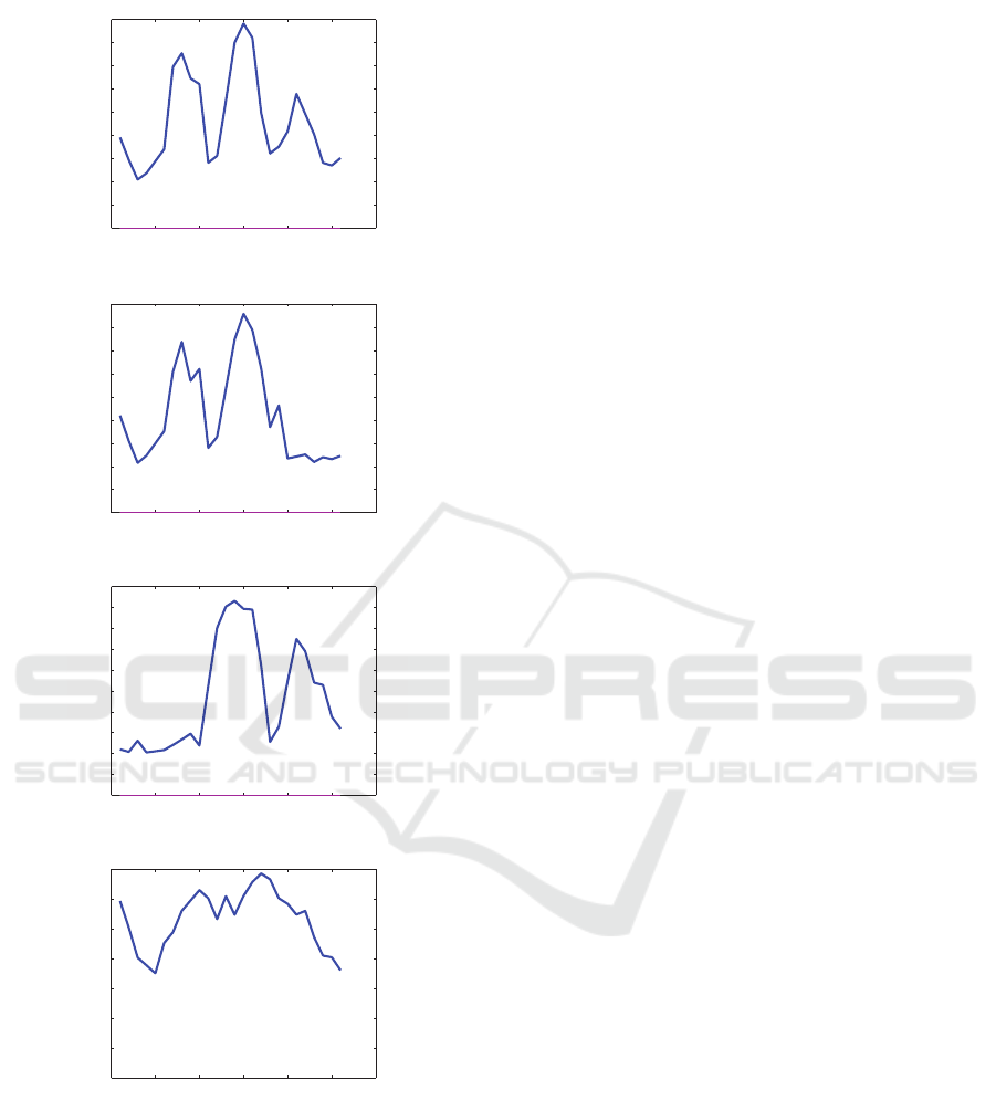
such as Agriculture. This deduction comes from the

fact that its MSE is relatively high (0.013) and this can

be explained by the heterogeneity of its class: it rep-

resents three behavior’s types as illutrated in Figure 7

and (Jonathan et al., 2005).

6 CONCLUSION

Thanks to coarse data, we conducted a clustering pro-

cess and generated ”labeled” dictionary. We explored

the sparse representation and its capabilities to ﬁt the

data, to reduce dimensions in order to improve clus-

tering results. We compared two classiﬁers : OMP

and SunSAL and found that SunSAL outperforms

OMP. But here some critics must be mentioned : al-

though MODIS images provide coverage at continen-

tal and global scales, the ability to reveal speciﬁc de-

tails of the region study remains difﬁcult. Many of

pixels generated by coarse resolution sensors are not

characteristic of only one vegetation but represent a

mixture as we mentioned in the experimentation sec-

tion. Therefore, for this study, we consider that the

pixel refers to one type of vegetation. So, in perspec-

tives, we aim to accurate our results by ﬁnding a way

to tradeoff multi-sensor data in order to enhance class

discrimination to monitor land cover change. This

would be done by the mean of merging multi-source

images with different spatial, spectral and temporal

resolutions.

RGB-SpectralImaging 2016 - Special Session on RBG and Spectral Imaging for Civil/Survey Engineering, Cultural, Environmental,

Industrial Applications

702

0 5 10 15 20 25 30

0.1

0.2

0.3

0.4

0.5

0.6

0.7

0.8

0.9

Dates

NDVI values

Agriculture

(a)

0 5 10 15 20 25 30

0.1

0.2

0.3

0.4

0.5

0.6

0.7

0.8

0.9

Dates

NDVI values

Agriculture

(b)

0 5 10 15 20 25 30

0.1

0.2

0.3

0.4

0.5

0.6

0.7

0.8

0.9

Dates

NDVI values

Agriculture

(c)

0 5 10 15 20 25 30

0.1

0.2

0.3

0.4

0.5

0.6

0.7

Dates

NDVI values

Agriculture

(d)

Figure 7: Ground truth temporal behaviors of Agriculture

Class. (a): Agriculture Temporal Behavior with 3 modes.

(b) and (c): Agriculture temporal behavior with 2 modes.

(d) : Agriculture Temporal Behavior with 1 mode.

ACKNOWLEDGEMENTS

The authors would thank the anonymous reviewers

for their helpful comments.

REFERENCES

Aharon, M., Elad, M., and Bruckstein, A. (2006). K-svd:

An algorithm for designing overcomplete dictionaries

for sparse representation. Signal Processing, IEEE

Transactions on, 54(11):4311–4322.

Bioucas-Dias, J. M. and Figueiredo, M. A. (2010). Alternat-

ing direction algorithms for constrained sparse regres-

sion: Application to hyperspectral unmixing. In Hy-

perspectral Image and Signal Processing: Evolution

in Remote Sensing (WHISPERS), 2010 2nd Workshop

on, pages 1–4. IEEE.

Brown, J. C., Kastens, J. H., Coutinho, A. C., de Castro Vic-

toria, D., and Bishop, C. R. (2013). Classifying mul-

tiyear agricultural land use data from mato grosso us-

ing time-series modis vegetation index data. Remote

Sensing of Environment, 130:39–50.

Chen, S. and Donoho, D. (1994). Basis pursuit. In Sig-

nals, Systems and Computers, 1994. 1994 Conference

Record of the Twenty-Eighth Asilomar Conference on,

volume 1, pages 41–44. IEEE.

Guha, T. and Ward, R. K. (2012). Learning sparse represen-

tations for human action recognition. Pattern Analy-

sis and Machine Intelligence, IEEE Transactions on,

34(8):1576–1588.

Jia, K., Wu, B., and Li, Q. (2013). Crop classiﬁcation using

hj satellite multispectral data in the north china plain.

Journal of Applied Remote Sensing, 7(1):073576–

073576.

Jonathan, M., Meirelles, M. S. P., Berroir, J.-P., Herlin,

I., and da Costa Coutinho, H. L. (2005). Regional

scale land use/land cover classiﬁcation using tempo-

ral series of modis data at the high taquari basin, ms,

brazil. Simp

osio Brasileiro de Sensoriamento Remoto,

12:579–581.

Lim, Y., Shinn-Cunningham, B., and Gardner, T. J. (2012).

Sparse contour representations of sound. Signal Pro-

cessing Letters, IEEE, 19(10):684–687.

Mahmoudi, M. and Sapiro, G. (2012). Sparse representa-

tions for range data restoration. IEEE transactions on

image processing: a publication of the IEEE Signal

Processing Society, 21(5):2909–2915.

Mohammady, M., Moradi, H., Zeinivand, H., and Temme,

A. (2015). A comparison of supervised, unsupervised

and synthetic land use classiﬁcation methods in the

north of iran. International Journal of Environmental

Science and Technology, 12(5):1515–1526.

Morton, D. C., DeFries, R. S., Shimabukuro, Y. E., An-

derson, L. O., Del Bon Esp

ırito-Santo, F., Hansen,

M., and Carroll, M. (2005). Rapid assessment of

annual deforestation in the brazilian amazon using

modis data. Earth Interactions, 9(8):1–22.

Rousseeuw, P. J. (1987). Silhouettes: a graphical aid to

the interpretation and validation of cluster analysis.

Journal of computational and applied mathematics,

20:53–65.

Tropp, J., Gilbert, A. C., et al. (2007). Signal recovery

from random measurements via orthogonal matching

pursuit. Information Theory, IEEE Transactions on,

53(12):4655–4666.

Land Cover Clustering based on Improved Dictionary Learning Method from Modis Data

703

Wright, J., Yang, A. Y., Ganesh, A., Sastry, S. S., and Ma,

Y. (2009). Robust face recognition via sparse repre-

sentation. Pattern Analysis and Machine Intelligence,

IEEE Transactions on, 31(2):210–227.

Xue, Z., Li, J., Cheng, L., and Du, P. (2015). Spectral–

spatial classiﬁcation of hyperspectral data via mor-

phological component analysis-based image separa-

tion. Geoscience and Remote Sensing, IEEE Trans-

actions on, 53(1):70–84.

Yang, X., Yang, T., Ji, Q., He, Y., and Ghebrezgabher,

M. G. (2014). Regional-scale grassland classiﬁca-

tion using moderate-resolution imaging spectrometer

datasets based on multistep unsupervised classiﬁca-

tion and indices suitability analysis. Journal of Ap-

plied Remote Sensing, 8(1):083548–083548.

Zhan, X., Sohlberg, R., Townshend, J., DiMiceli, C.,

Carroll, M., Eastman, J., Hansen, M., and DeFries,

R. (2002). Detection of land cover changes using

modis 250 m data. Remote Sensing of Environment,

83(1):336–350.

RGB-SpectralImaging 2016 - Special Session on RBG and Spectral Imaging for Civil/Survey Engineering, Cultural, Environmental,

Industrial Applications

704