Individual Mobility Patterns in Urban Environment
Pierpaolo Mastroianni
1
, Bernardo Monechi
2
, Vito D. P. Servedio
3,4
, Carlo Liberto
1
, Gaetano Valenti
1
and Vittorio Loreto
3,2
1
ENEA, Casaccia Research Center, Via Anguillarese 301, 00123, Rome, Italy
2
Institute for Scientific Interchange Foundation, Via Alassio 11/c, 10126, Turin, Italy
3
Sapienza University of Rome, Physics Dept., P.le Aldo Moro 2, 00185 Roma, Italy
4
Institute for Complex Systems (ISC-CNR), Via dei Taurini 19, 00185 Roma, Italy
Keywords:
Urban Mobility, Daily Patterns, Optimization, Circadian Rhythm.
Abstract:
The understanding and the characterization of individual mobility patterns in urban environments is important
in order to improve liveability and planning of big cities. In relatively recent times, the availability of data
regarding human movements have fostered the emergence of a new branch of social studies, with the aim
to unveil and study those patterns thanks to data collected by means of geolocalization technologies. In this
paper we analyze a large dataset of GPS tracks of cars collected in Rome (Italy). Dividing the drivers in
classes according to the number of trips they perform in a day, we show that the sequence of the traveled
space connecting two consecutive stops shows a precise behavior so that the shortest trips are performed at the
middle of the sequence, when the longest occur at the beginning and at the end when drivers head back home.
We show that this behavior is consistent with the idea of an optimization process in which the total travel time
is minimized, under the effect of spatial constraints so that the starting points is on the border of the space in
which the dynamics takes place.
1 INTRODUCTION
The spreading of ICT (Information and Communica-
tion Technology) devices across the population has
led to the unprecedented possibility to monitor the
daily activity of citizen’s in almost real time (Mayer-
Schonberger and Cukier, 2013). Despite privacy is-
sues (Tene and Polonetsky, 2012; Rubinstein, 2013),
these new technology are of utmost importance in so-
cial science studies, since they are opening the pos-
sibility for a better understanding of large-scale col-
lective phenomena (Gonzalez-Bailon, 2013; Lazer
et al., 2009; Eluru et al., 2009). Among the possi-
bility offered by the large availability of human activ-
ity data, the study of how people move and interact
within a urban environment could give an important
contribute to the future social challenges in terms of
reducing pollution and increase the livability of big
cities (United Nations Secretariat, 2014). Moreover,
the study of other phenomena like epidemic spread-
ing(Eubank et al., 2004; Colizza et al., 2007) can-
not abstract from the understanding of human mobil-
ity. For these reasons, many relatively recent works
have focused on the derivation of universal statistical
laws characterizing the patterns of human movements
(Brockmann et al., 2006; Gonzalez et al., 2008; Song
et al., 2010; Simini et al., 2012; Wang et al., 2014).
In this paper we address the problem of the charac-
terization of the daily patterns of car drivers, in order
to understand how they move between different areas
of the city during each day. Similarly to other works
(Bazzani et al., 2010; Gallotti et al., 2012; Rambaldi
et al., 2007; Gallotti, 2013; Gallotti et al., 2015), we
analyze a large database of GPS tracks of private cars
collected in the Rome (Italy) district during the whole
month of May 2011. The study of the dynamics of car
travel has a long tradition in Complex Systems and
Physics framework, modelling traffic flows from both
an Eulerian and Lagrangian perspectives (Treiber and
Kesting, 2013; Rambaldi et al., 2007). Our findings
suggest that there is a universal pattern in the way
drivers choose the sequence of places they have to
visit, so that independently of their number the se-
quence of the length of the trips connecting them has
a “parabolic” shape. Note that a similar approach has
been used also considering mobile phone data (Cal-
abrese et al., 2013), which is a proxy for multi-modal
mobility, i.e. all the possible kind of means of trans-
Mastroianni, P., Monechi, B., Servedio, V., Liberto, C., Valenti, G. and Loreto, V.
Individual Mobility Patterns in Urban Environment.
In Proceedings of the 1st International Conference on Complex Information Systems (COMPLEXIS 2016), pages 81-88
ISBN: 978-989-758-181-6
Copyright
c
 2016 by SCITEPRESS – Science and Technology Publications, Lda. All rights reserved
81

portation are considered. By means of a model intro-
duced in (Mastroianni et al., 2015), we show how this
pattern can emerge from the interplay between the ge-
ometric constraints of the space in which the stops are
placed and the need to optimize the overall travel time
in order to get back to the starting point at the end of
the day.
2 GPS TRACKS DATA AND DAILY
DYNAMICS PATTENRS
2.1 Data
Approximately 4% and 8% of the whole vehicle pop-
ulation inside the Rome (Italy) district during the
months of May 2011 and May 2013, respectively, was
monitored on behalf of an insurance company (Oct,
2014). For that, time, position, velocity and covered
distance of single vehicles were recorded by sampling
each trajectory at a time scale of 30 seconds (on fast
speed roads, e.g., on highways) or at a spatial scale of
2km (elsewhere). This sampling strategy was chosen
by that company to ensure a better sampling rate on
arterial roads. A further signal was also recorded each
time the engine was switched on or off so that a travel
is defined as the temporal ordered sequence of points
between the engine start and stop. Due to privacy is-
sues, it is not possible to know any information about
the owner of the vehicle performing the trips. Hence,
in the following we do not distinguish between private
or professional drivers, nor the reasons why a trip has
been performed. In total, we are able to study the
spatial pattern of 13,527 vehicles during 20 working
days with an average number of trips per day equal to
11,524. Errors due to GPS signal quality have been
already considered in (Mastroianni et al., 2015), we
refer to this work for details. We consider as the same
trip, two consecutive journeys performed by the same
car if the stop time between them, i.e. the difference
between the switch off time of the engine at the end
of the first trip and the switch on time at the beginning
of the second, is smaller than 5 minutes. The distri-
bution P(n) of the number n of trips performed by a
driver during a day can be approximated for n ≥ 5 by
an exponential law with a typical length n
0
= 2.51(2)
as displayed in Fig. 1. The trips made up by a small
number of stops clearly dominate overall our sample.
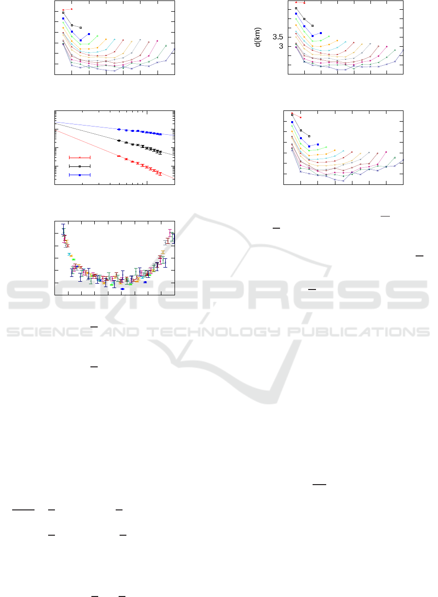
2.2 Parabolic Pattern of Trips
Considering the sequence of the n trips performed in
a day by the same driver it is possible to define the
10
-4
10
-3
10
-2
10
-1
10
0
0 2 4 6 8 10 12 14 16 18
P(n)
n
n
0
=2.51(2)
Figure 1: Distribution of the number of trips n performed
by a driver in each day. Black line represents the best fit
with an exponential function ∝ exp(−
n
n
0
).
quantity l
n
k
, i.e., the distance traveled during the k
th
trips. We can then compute
l
n
k
by averaging over all
the k
th
of the drivers with n movements. This op-
eration of average might hide the differences inside
the sample it makes regular patterns emerge from the
data. If the way in which each driver chooses the se-
quence of stops performed during a day would be ran-
dom, the sequence of
l
n
k
would not depend on k. In-
stead they follow the behavior in Fig. 2 panel a. For
every value of n, the sequence of
l
n
k
strongly depends
on k. Moreover, the sequence of
l
n
k
seems to be par-
ticularly regular being symmetric around k =
(n+1)
2
,
where it reaches its minimum value. Thus,
l
n
k
de-
creases starting from k = 0 until k =
(n+1)
2
is reached,
then starts growing again until k = n. Note that
l
n
0
and
l
n
n
are the highest values of the sequence and their val-
ues become more similar as n grows. This suggests
that for each n,
l
n
k
can be approximated by a parabola,
whose coefficients depend on n:
p
n
(k) = a
n
k
2
+ b
n
k+ c
n
. (1)
For every value of n, p
n
(k) is a parabola with sym-
metry axis orthogonal to the k axis. Fitting p
n
(k)
by means of the sequence
l
n
k
with the corresponding
value of n, the coefficients a
n
, b
n
and c
n
grow with n
as a power-law (Fig. 2 panel b).
Thus it is possible to write:
a
n
= An
−η
a
b
n
= Bn
−η
b
c
n
= Cn
−η
c
.
(2)
where A = 8.8(7)Km, B = 21(1)Km,
C = 24.5(8)Km, η
a
= 2.00(4), η
b
= 1.33(4)
and η
c
= 0.55(2). Thus, combining equations (1) and
(2),
p
n
(k) = An
−η
a
k
2
+ Bn
−η
b
k+Cn
−η
c
. (3)
Dividing each members of (3) by Cn
−η
c
, we get
p
n
(k)
c
n
=
A
C
n
−(η
a
−η
c
)
k
2
+
B
C
n
−(η
b
−η
c
)
k+ 1. (4)
COMPLEXIS 2016 - 1st International Conference on Complex Information Systems
82

3
4
5
6
7
8
9
10
0 2 4 6 8 10 12 14
l(km)
k
a)
10
-2
10
-1
10
0
10
1
10
2
1 10
n
l(km)
b)
a
n
b
n
c
n
10
-1
10
-1
10
-1
10
-1
10
-1
10
0
10
0
0 0.2 0.4 0.6 0.8 1 1.2 1.4 1.6 1.8
l(km)
k
c)
Figure 2: (a) sequences l
n
k
for some values of n. Differ-
ent colors correspond to different values of the number of
trips n. (b) sequences of the coefficients of the parabolic fit
p
n
(k) for n ≥ 4. Continuous lines are power law fit of the
sequences. (c) sequences
l
n
k
divided by c
n
as functions of
ˆ
k.
Note that with the estimated values of the parameters,
η
a
− η
c
= 1.45(4)
η
b
− η
c
= 0.78(4).
(5)
This indicates that, within the estimated errors, the
following relation holds
η
a
− η
c
= 2(η
b
− η
c
). (6)
The relation (6) allows to derive a scaling law for
equation (3). In fact
p
n
(k)
c
n
=
A
C
n
−2(η
b
−η
c
)
k
2
+
B
C
n
−(η
b
−η
c
)
k+ 1
=
A
C
(n
−(η
b
−η
c
)
k)
2
+
B
C
n
−(η
b
−η
c
)
k+ 1.
(7)
Then it is possible to define a new variable
ˆ
k =
n
−(η
b
−η
c
)
k, obtaining a universal expression for the
parabola independent of n
p(
ˆ
k) =
A
C
ˆ
k
2
+
B
C
ˆ
k+ 1. (8)
1.5
2
2.5
4
4.5
5
5.5
0 2 4 6 8 10 12 14
k
a)
10
12
14
16
18
20
22
24
0 2 4 6 8 10 12 14
t(min)
k
b)
Figure 3: sequences of euclidean distances d
n
k
(panel a) and
travel times
t
n
k
(panel b) for some values of n.
This indicates that rescaling all the values of l
n
k
by
c
n
, all the data would collapse over the curve defined
by Eq. (8). Fig. 2 in panel c shows the collapse of
the data for all the
l
n
k
sequences. The variability of
the data, combined with the parabolic approximation
used, does not provide a very precise collapse but the
indication of a universal scaling law still holds. Sim-
ilar properties can also be found for the sequence of
the euclidean distances between subsequent stops d
n
k
and for the sequence of the travel times t
n
k
. Their cor-
responding parabolas are shown in Fig. 3. Despite the
approximation of the parabolic fit, some general fea-
tures can be identified for all the previously presented
sequences. Independently of the value of n, the first
value of the sequence with k = 1 is the largest one.
Apart from n = 2 and n = 3, all the sequences are ini-
tially decreasing until a certain value of k, say k
∗
n
, is
reached. Around k = k
∗
n
the sequences reach a mini-
mum, then for k > k
∗
n
they start growing with k. As n
grows, the value of k
∗
n
gets closer to the central value
of the sequence k =
n+1
2
. Since the dynamics of the
individual is certainly related to the circadian rhythm,
the emergence of these parabolic pattern are probably
related to the constraint of going back to the origin of
the trip.
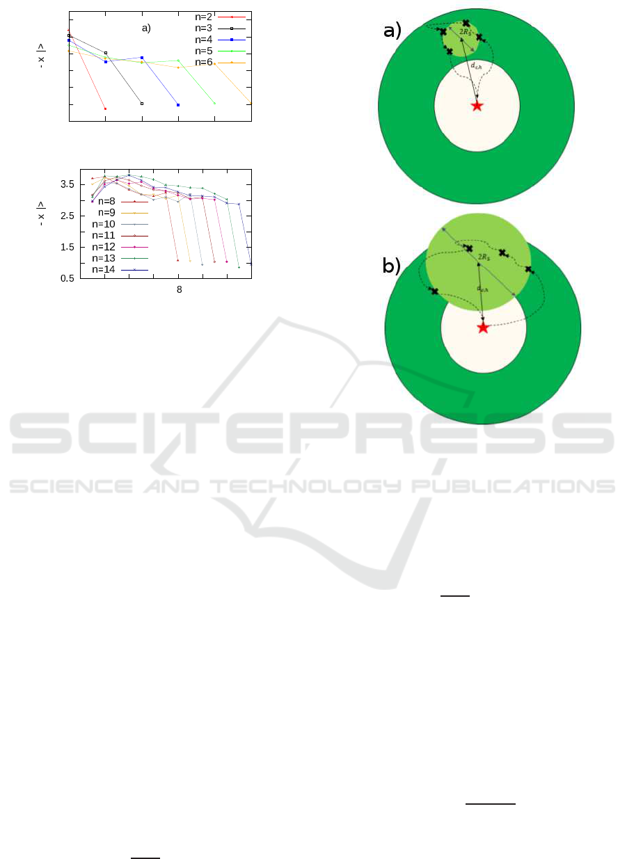
2.3 Spatial Constraints on Daily Stops
Indicating with~x
k
the coordinates of the k-th stops of
a driver, we can consider the point ~x
0
as the starting
point of the daily dynamics and study the spatial rela-
Individual Mobility Patterns in Urban Environment
83

0
1
2
3
4
5
6
1 2 3 4 5 6
<|x
k 0
k
1
2
3
4
0 2 4 6 10 12 14
<|x
k 0
k
b)
Figure 4: sequences d
n
(~x
k
,~x
0
) of the average distances from
the starting point.
tions between it and the other points k ∈ [1, n]. Con-
sidering all the sequences with the same number of
trips n, we can define the sequence of average dis-
tances between the k-th stop and the starting point
d
n
(~x
k
,~x
0
) = h|~x
k
−~x
0
|i, where |.| indicates the eu-
clidean distance. Fig. 4 shows these values for some
value of the number of trips per day n. It is evident
how the distance between the last point and the first
one is usually smaller with respect to the others, indi-
cating that usually at the end of the dynamics drivers
tend to go back to the starting point. However this
final distance is between 0.5km and 1km, so that the
final point does not coincide exactly with the first one.
The fact that the distance between the initial and the
other stops was usually constant suggested two kinds
of possible dynamics for the choice of the sequence
of the stops: an orbital dynamics and a bipolar dy-
namics, depicted in Fig. 5. In the orbital dynamics
the stops are disposed at a constant radius around the
origin. In the other case the driver performs a long
movement and then a series of shorter movements.
These movements are so that the distances between
the points they connect and the origin are quite con-
stant so that they are displaced on average over a cir-
cular arc centered in the origin. The last movement
is again a long one in order to get back to the origin.
In order to discriminate between these two dynamics,
we consider the barycenter of the intermediate stops
(i.e. with k 6= 0 and k 6= n)
~r
c
=
1
n− 1
n−1
∑
k=1
~x
k
. (9)
Figure 5: Representations of an orbital (a) and bipolar (b)
dynamics for a driver performing 4 stops. In (a) the ra-
dius of gyration R
5
is comparable to the distance between
the origin and the barycenter d
c,h
since the points are rather
scattered, thus leading to ρ
5
> 0. On the contrary in (b) the
points are quite clustered around the barycenter and thus
ρ
5
< 0.
The gyration radius around this point is
R
2
n
=
1
n− 1
n−1
∑
k=1
|~x
k
−~r
c
|
2
, (10)
measuring how much the dispersion of the intermedi-
ate stops around their barycenter. We can also define
the quantity d
c,h
= |~r
c
−~x
0
|, i.e. the distance between
the starting point and the barycenter. If R
n
< d
c,h
,
then the dispersion of the intermediate points will be
smaller than the distance between the starting point
and their barycenter, resulting in a bipolar dynamics.
The opposite condition will indicate instead an orbital
dynamics. To summarize these conditions with an
adimensional metrics, we define
ρ
n
=
R
n
− d
c,h
R
n
+ d
c,h
, (11)
which is bounded between −1 and 1, so that ρ
n
< 0
and ρ
n
> 0 correspond respectively to the bipolar and
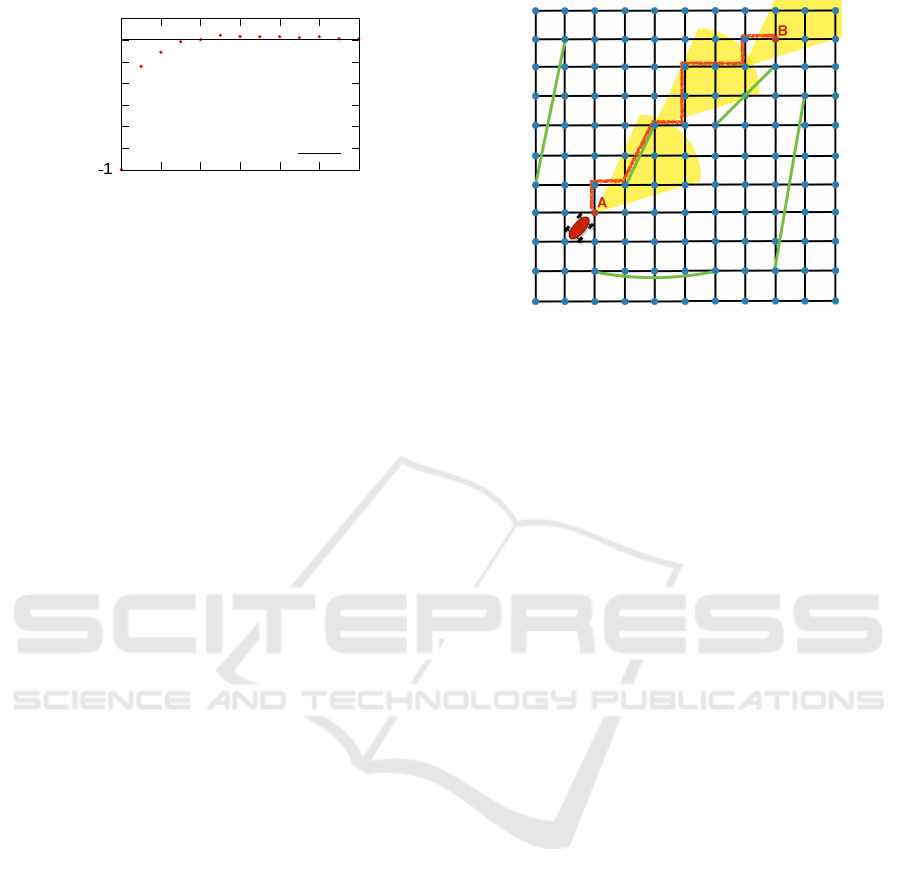
orbital dynamics. Fig. 6 shows the average values of
COMPLEXIS 2016 - 1st International Conference on Complex Information Systems
84

-0.8
-0.6
-0.4
-0.2
0
0.2
0.4
2 4 6 8 10 12 14
ρ
n
n
0.209(2)
Figure 6: sequences ρ
n
. The horizontal black line is the best
fit of a constant function for points with n > 4.
R
n
as function of n. For n ≥ 5, R
n
has a constant value
of 0.209(2), while for n < 5 its values are smaller but
still larger than 0. The only exception is represented
by the point n = 3 which is slightly smaller than 0,
and the point n = 2 which is equal to −1 by definition
since R
2
= 0. Hence, the orbital dynamics seems to be
the dominant one across the whole sample of tracks.
3 DAILY DYNAMICS AS
CONSTRAINED
OPTIMIZATION
3.1 Modeling Road Network
In (Mastroianni et al., 2015) we have introduced a
simple model of road network, where the regular
roads of the city were represented as an N × N grid
whose links were of unit length and that could be trav-
eled at constant unit speed. We introduced a certain
number N
shortcut
of additional links connecting ran-
dom nodes of the grid, that could be traveled at a
higher speed v > 1 and their length was the euclidean
distance between the nodes. These longer links repre-
sented arterial roads exploited by car driver in order to
cross rapidly the urban environment. We showed how
the interplay between the arterial roads and the ability
of the car drivers to optimally choose the path con-
necting the origin and the destination of a trip (i.e.,
minimizing the travel time), was able to explain the
sub-linear growth of the average speed during a trip
with the total trip length. However, in order to repro-
duce the correct paths the optimization has to be sub-
optimal: we supposed that the drivers are not able to
choose the globally optimal path due to their limited
knowledge of the urban environment, but can opti-
mize it piece-wise between known locations until the
car reach their destination. Thus, we defined a Navi-
gation Algorithm (NA) depicted in Fig. 7. Assuming
that a driver must go from the node A to the node B
Figure 7: Representation of the Grid Network with short-
cuts (green links) and of the Navigation Algorithm used to
build synthetic paths connecting the nodes A and B.
of the grid, the navigation algorithm proceeds as fol-
lows:
• Assuming that the current node visited by the al-
gorithm at its i
th
step is n
i
, we choose an opti-
mization distance l
optim
from a uniform distribu-
tion in [3, l(n
i
,B)], where l(n
i
,B) is the euclidean
distance between n
i
and B.
• The next visited node n
i+1
is chosen randomly be-
tween all the nodes whose distance from n
i
is less
than l
optim
. Moreover, the angle between the lines
connecting n
i
and n
i+1
and A and B is smaller than
an assigned value α (α = 30
o
in the following).
• If B satisfies the conditions in the previous point,
it is automatically chosen as n
i+1
• If n
i+1
= B the process ends.
Once a sequence of nodes {A, n
1
,n
2
,...,B} is made
with the algorithm, the path connecting A and B is
built by concatenating all the shortest paths connect-
ing each n
i
with its successive node n
i+1
. In the next
paragraph we used the NA and our urban network
model to build some synthetic paths and studied how
the parabolic patterns might emerge from a sequence
of trips.
3.2 The Traveling Salesman
We have seen how the sequence of trips performed
by a driver is linked to his circadian rhythm, since
the last one is usually performed to go back to his
initial location. Moreover, the sequence of stops is
chosen according to an orbital dynamics, i.e., they are
deployed at a constant radius around the origin. Thus,
we can use this information to build a model that can
reproduce these patterns in a simple way. By using
our grid model and the NA, we assume that a driver
Individual Mobility Patterns in Urban Environment
85

starts his daily dynamics from node i
start
and has to
perform other n−1 stops before going back home. He
may choose this node randomly from all the nodes in
the grid, but we this choice is fundamental in order to
obtain the desired pattern. Practically, the algorithm
defining the sequence proceeds as follows:
• We choose n − 1 distinct nodes as intermediate
stops. These nodes are chosen randomly between
all the nodes in the grid.
• We build a path connecting each pair of stops i
and j (including i
start
) using the navigation algo-
rithm. Thus, we construct the matrix t
i, j
of the
travel times of the paths connecting every pair of
stops.
• The sequence of stops {i
start
,i
1
,i
2
,...,i
n−1
,i
start
}
is then the one that minimizes the total travel time,
i.e.,
T =
n−1
∑
k=0
t
i
k
,i
k+1
, (12)
where i
0
= i
n
= i
start
.
• At the end of the procedure we have the optimal
sequences d
n
k
, t
n
k
and l
n
k
.
Note that this procedure would be equivalent to the
Traveling Salesman Problem (Flood, 1956) on the
grid with shortcuts if the shortest path between two
successive nodes would have been chosen instead of
the one build with the navigation algorithm. In the
following, we sampled more than 2,000 paths for each
value of n and N
shortcut
in the grid model, and com-
puted
d
n
k
, t
n
k
and l
n
k
. For each path, the shortcuts are
reassigned over the grid. The speed on the links in the
grid and in the shortcuts has been chosen as constant,
with values of 1 and 2 respectively. Different choices
lead to qualitatively similar results. The first check
that can be made is that the choice of i
start
must not be
random.
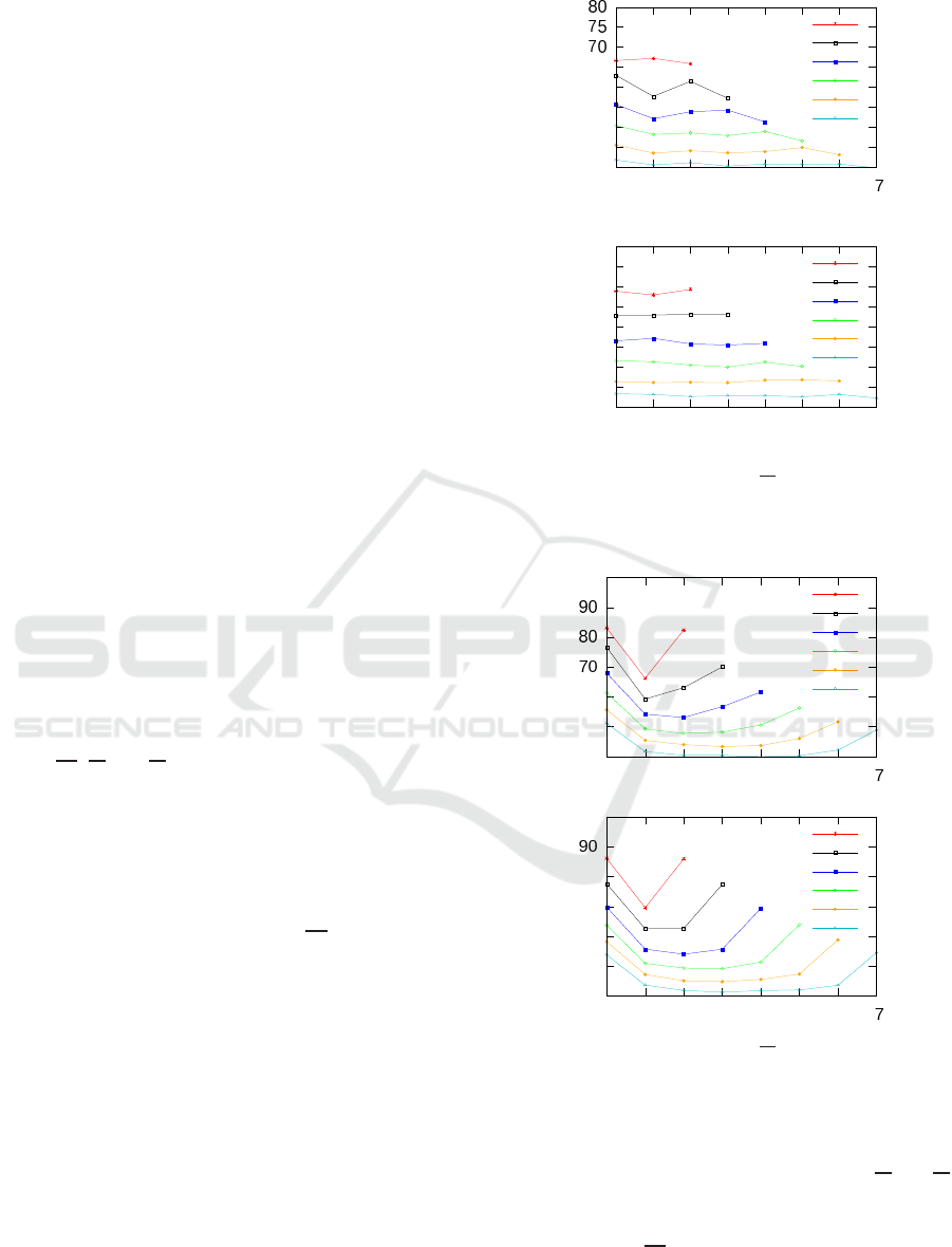
Fig. 8 shows the sequences of
d
n
k
for some val-
ues of n in grids with L = 100 and N
shortcuts
= 0 and
N
shortcuts
= 100. The values of the sequence as n in-
creases are quite constant or follow an irregular pat-
tern, rather different from the one observed in the
data. Fig. 9 shows the same sequences with i
start
cho-
sen randomly at the border of the grid. In this case it
is evident that the sequences show the desired behav-
ior: an initial decrease towards a minimum and then
an increase until a value similar to the initial one is
reached. This indicates that the interplay between the
optimization process and the confined geometry of the
urban environment is crucial in order to understand
how the observed patterns emerge. The “parabola-
like” sequence seems to be the results of an optimiza-
tion process performed within a limited area, starting
40
45
50
55
60
65
0 1 2 3 4 5 6
l(adim.)
k
a)
n=3
n=4
n=5
n=6
n=7
n=8
40
45
50
55
60
65
70
75
80
0 1 2 3 4 5 6 7
l(adim.)
k
b)
n=3
n=4
n=5
n=6
n=7
n=8
Figure 8: Sequence of trip lengths l
n
k
on the grid model with
N
shortcuts
= 0 (a) and N
shortcuts
= 100 (b) when the origin of
the trips is randomly chosen on the grid.
40
50
60
100
0 1 2 3 4 5 6
l(adim.)
k
a)
n=3
n=4
n=5
n=6
n=7
n=8
40
50
60
70
80
100
0 1 2 3 4 5 6
l(adim.)
k
b)
n=3
n=4
n=5
n=6
n=7
n=8
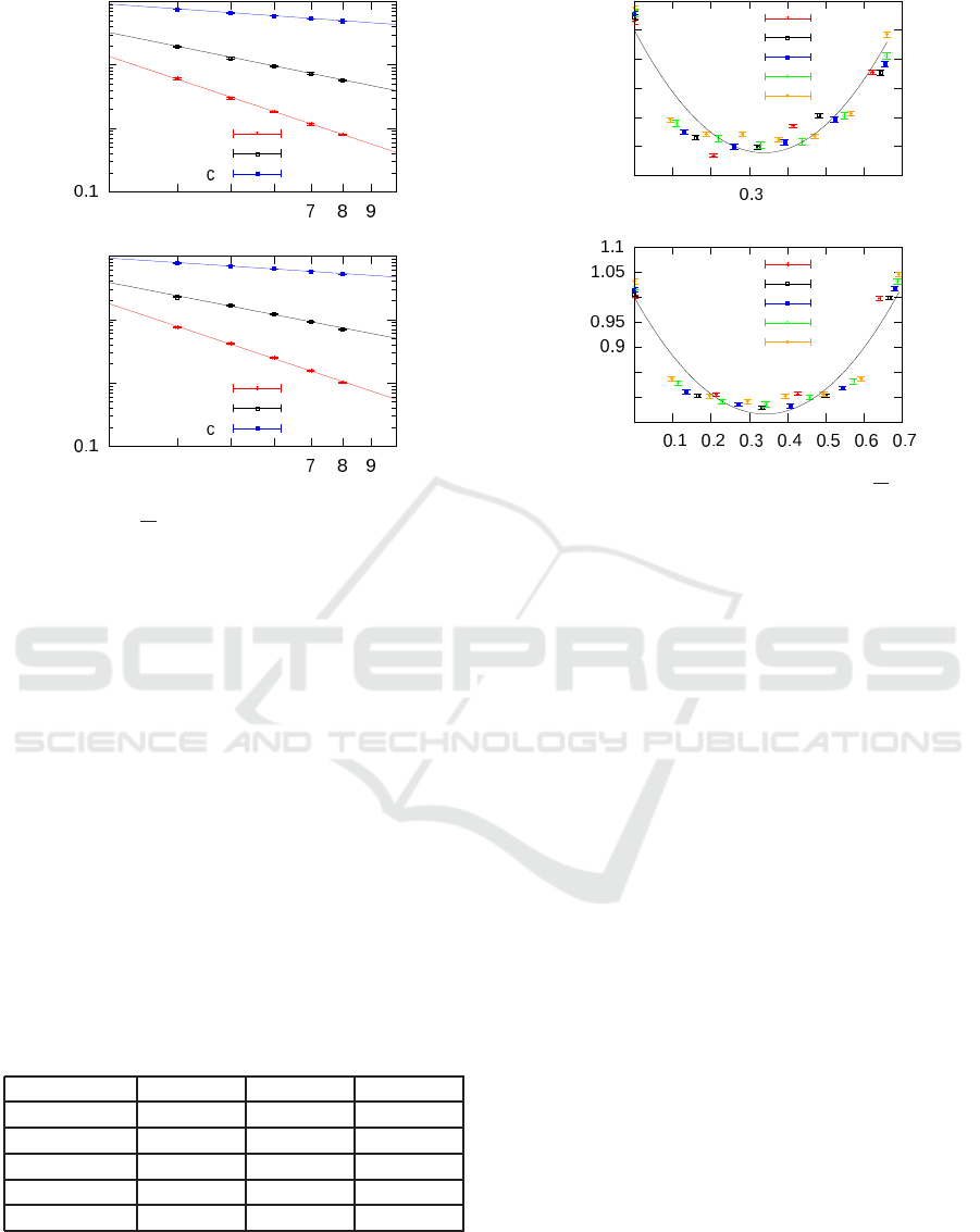
Figure 9: Sequence of trip lengths l
n
k
on the grid model with
N
shortcuts
= 0 (a) and N
shortcuts
= 100 (b) when the origin of
the trips is randomly chosen at the border of the grid.
from a point close to the boundaries of such area.
Note that, as we have seen in the data, also
t
n
k
and l
n
k
possess this kind of structure (Fig. 3).
In Section 2.2 it has been shown that approximating
the sequence of
d
n
k
with a parabola p
n
(k) it is pos-
sible to derive a scaling law for the sequence. De-
spite the fact that in our case the parabolic fit does
COMPLEXIS 2016 - 1st International Conference on Complex Information Systems
86

1
10
100
3 4 5 6 10
l(adim.)
n
a)
a
n
b
n
n
1
10
100
3 4 5 6 10
l(adim.)
n
b)
a
n
b
n
n
Figure 10: Coefficients a
n
, b
n
and c
n
of the parabolic fit
for the sequence
l
n
k
for some values of n on the grid with
N
shortcuts
= 0 (a) and N
shortcuts
= 100 (b). Continuous lines
are power-law fits of the points.
not describe well the sequence, we can still use it in
order to see if there is a similar scaling also for the
sequences on the grid. Therefore, we fit the curves
in Fig. 9 with Eq. (1). In both cases we check that
the coefficients p
n
(k) are power-law decreasing with
n, so that equations (2) hold (see Fig. 10). Moreover,
also the relations between the coefficients in Eq. (6)
is still valid even though the approximation is worse
for N
shortcuts
= 100 (Table 1 displays the values of the
exponents of Eq. 2 for some values of N
shortcuts
).
Fig. 10 shows the collapsed sequences together
with the universal parabola independent from n. It
is evident that, despite a scaling law seems to exist,
the parabola does not describe well the curves since
the found behavior shows a smaller curvature.
Table 1: Values of the exponents of Eq. (2) inferred from
the grid model.
N
shortcuts
0 50 100
η
a
2.89(8) 2.91(7) 2.95(5)
η
b
1.76(8) 1.72(8) 1.74(5)
η
c
0.62(1) 0.58(2) 0.58(2)
η
c
− η
a
−2.26(1) −2.34(9) −2.30(7)
2(dη
c
− η
b
) −2.27(1) −2.3(2) −2.32(7)
0.75
0.8
0.85
0.9
0.95
1
1.05
0 0.1 0.2 0.4 0.5 0.6 0.7
l(adim.)
k
a)
n=4
n=5
n=6
n=7
n=8
0.75
0.8
0.85
1
0
l(adim.)
k
b)
n=4
n=5
n=6
n=7
n=8
Figure 11: Collapsed sequence of trip lengths l
n
k
on the grid
model with N
shortcuts
= 0 (a) and N
shortcuts
= 100 (b) when
the origin of the trips is randomly chosen on the border of
the grid.
4 CONCLUSIONS
In this paper we analyzed a large dataset of GPS
tracks about vehicles collected within the city of
Rome. After dividing the drivers according to the
number of trips performed within a day, we showed
that the sequence of travel length, as well as the se-
quences of travel times and geodesic distances be-
tween stops, exhibit a “parabolic pattern” so that each
sequence is initially decreasing until a minimum is
reached and then grows again to another maximum.
By fitting these sequences with a parabolic law we
showed that each one can be rescaled in a universal
form independent from the number of trips, suggest-
ing the existence of a universal mechanism responsi-
ble of this observed pattern. By using a model intro-
duced in (Mastroianni et al., 2015) to produce syn-
thetic paths in a simplified urban environment, we
showed that these findings are consistent with the idea
of drivers trying to minimize the total travel time. The
geometry of the problem seems to be crucial in order
to reproduce the correct behavior, so that the start-
ing point must be at the border of a space that con-
strains the dynamics. Despite the fact that the simu-
lated sequences of trip lengths are not well described
by parabolic laws, still the model exhibit a scaling law
similar to the one found empirically.
Despite the simplicity of the modeling scheme, the
empirical patterns found in the data are qualitatively
Individual Mobility Patterns in Urban Environment
87

reproduced. We argue that a more realistic model,
taking into account different traffic conditions could
lead to a better agreement with the data and a bet-
ter understanding on the behavioral changes of car
drivers. Finally, the universality of our findings have
still to be completely proven by performing similar
measurements in different urban environments and
time-frames. The observed patterns might be useful
in order to develop improved info-mobility systems
taking into account the possible behavior of a driver
on his next trip. The understanding of the behavior
of individual car movements could in fact help at im-
proving traffic forecast systems.
ACKNOWLEDGEMENTS
The authors acknowledge support from the KREYON
project funded by the Templeton Foundation under
contract n. 51663. VDPS acknowledges the EU FP7
Grant 611272 (project GROWTHCOM), the CNR
PNR Project “CRISIS Lab” for financial support. We
acknowledge interesting discussions with P. Gravino.
We thank M. Mancini for his valuable work on Oc-
toTelematics data pre-processing.
REFERENCES
Octotelematics. https://www.octotelematics.com/en/. Ac-
cessed: 2014-10-03.
Bazzani, A., Giorgini, B., Rambaldi, S., Gallotti, R., and
Giovannini, L. (2010). Statistical laws in urban mobil-
ity from microscopic gps data in the area of florence.
Journal of Statistical Mechanics: Theory and Experi-
ment, 2010(05):P05001.
Brockmann, D., Hufnagel, L., and Geisel, T. (2006). The
scaling laws of human travel. Nature, 439(7075):462–
465.
Calabrese, F., Diao, M., Di Lorenzo, G., Ferreira, J.,
and Ratti, C. (2013). Understanding individual mo-
bility patterns from urban sensing data: A mobile
phone trace example. Transportation research part C:
emerging technologies, 26:301–313.
Colizza, V., Barrat, A., Barth´elemy, M., Valleron, A. J.,
and Vespignani, A. (2007). Modeling the worldwide
spread of pandemic influenza: Baseline case and con-
tainment interventions. PLOS MEDICINE, 4(1):95–
110.
Eluru, N., Sener, I., Bhat, C., Pendyala, R., and Axhausen,
K. (2009). Understanding residential mobility: joint
model of the reason for residential relocation and stay
duration. Transportation Research Record: Journal of
the Transportation Research Board, (2133):64–74.
Eubank, H., Guclu, S., Kumar, V. S. A., Marathe, M.,
Srinivasan, A., Toroczkai, Z., and Wang, N. (2004).
Controlling Epidemics in Realistic Urban Social Net-
works. Nature, 429.
Flood, M. M. (1956). The traveling-salesman problem. Op-
erations Research, 4(1):61–75.
Gallotti, R. (2013). Statistical Physics and Modelling of Hu-
man Mobility. PhD thesis, Physics Department, Uni-
versity of Bologna.
Gallotti, R., Bazzani, A., and Rambaldi, S. (2012). Towards
a statistical physics of human mobility. International
Journal of Modern Physics C, 23(09):1250061.
Gallotti, R., Bazzani, A., and Rambaldi, S. (2015). Un-
derstanding the variability of daily travel-time expen-
ditures using gps trajectory data. EPJ Data Science,
4(1):1–14.
Gonzalez, M. C., Hidalgo, C. A., and Barabasi, A.-L.
(2008). Understanding individual human mobility
patterns. Nature, 453(7196):779–782.
Gonzalez-Bailon, S. (2013). Social Science in the Era of
Big Data. Social Science Research Network Working
Paper Series.
Lazer, D., Pentland, A., Adamic, L., Aral, S., Barab´asi, A.-
L., Brewer, D., Christakis, N., Contractor, N., Fowler,
J., Gutmann, M., Jebara, T., King, G., Macy, M., Roy,
D., and Van Alstyne, M. (2009). Computational social
science. Science, 323(5915):721–723.
Mastroianni, P., Monechi, B., Liberto, C., Valenti, G.,
Servedio, V. D. P., and Loreto, V. (2015). Local opti-
mization strategies in urban vehicular mobility. PLoS
ONE, 10(12):e0143799.
Mayer-Schonberger, V. and Cukier, K. (2013). Big Data: A
Revolution That Will Transform How We Live, Work,
and Think. Houghton Mifflin Harcourt, Boston.
Rambaldi, S., Bazzani, A., Giorgini, B., , and Giovannini,
L. (2007). Mobility in modern cities: Looking for
physical laws. In Proceedings of the European Con-
ference on Complex Systems, Dresden. ECCS07.
Rubinstein, I. S. (2013). Big Data: The End of Privacy or
a New Beginning? International Data Privacy Law.
im Erscheinen, NYU School of Law, Public Law Re-
search Paper Nr. 12-56.
Simini, F., Gonz´alez, M. C., Maritan, A., and Barab´asi, A.-
L. (2012). A universal model for mobility and migra-
tion patterns. Nature, 484(7392):96–100.
Song, C., Koren, T., Wang, P., and Barabasi, A.-L. (2010).
Modelling the scaling properties of human mobility.
Nature Physics, 6(10):818–823.
Tene, O. and Polonetsky, J. (2012). Big Data for All: Pri-
vacy and User Control in the Age of Analytics. North-
western Journal of Technology and Intellectual Prop-
erty.
Treiber, M. and Kesting, A. (2013). Traffic flow dynamics.
Traffic Flow Dynamics: Data, Models and Simulation,
Springer-Verlag Berlin Heidelberg.
United Nations Secretariat (2014). World urbanization
prospects: The 2014 revision. Technical report, De-
partment of Economic and Social Affairs.
Wang, X.-W., Han, X.-P., and Wang, B.-H. (2014). Correla-
tions and scaling laws in human mobility. PLoS ONE,
9(1):e84954.
COMPLEXIS 2016 - 1st International Conference on Complex Information Systems
88