
Contour Learning and Diffusive Processes for Colour Perception
Francisco J. Diaz-Pernas, Mario Martínez-Zarzuela, Miriam Anton-Rodriguez
and David González-Ortega
Imaging and Telematics Group, University of Valladolid, Campus Miguel Delibes, 47011, Valladolid, Spain
Keywords: Computer Vision, Contour Learning, Boundary Detection, Neural Networks, Colour Image Processing, Bio-
Inspired Models.
Abstract: This work proposes a bio-inspired neural architecture called L-PREEN (Learning and Perceptual boundaRy
rEcurrent dEtection neural architecture). L-PREEN has three different feedback interactions that fuse the
bottom-up and top-down contour information of visual areas V1-V2-V4-Infero Temporal. This recurrent
model uses colour, texture, and diffusive features to generate surface perception and contour learning and
recognition processes. We compare the L-PREEN model against other boundary detection methods using the
Berkeley Segmentation Dataset and Benchmark (Martin et al., 2001). The results obtained show better
performance of L-PREEN using quantitative measures.
1 INTRODUCTION
In this paper, a bio-inspired neural architecture called
L-PREEN (Learning and Perceptual boundaRy
rEcurrent dEtection Neural architecture) is proposed.
L-PREEN has three different feedback interactions
that fuse the bottom-up and top-down contour
information of visual areas V1-V2-V4-IT. This
recurrent model uses colour, texture and diffusive
features to generate diffusive surface perception and
contour learning processes.
There are several artificial neural models that
model the behaviour of the human system (Grossberg
and Williamson, 1999), (Kokkinos et al., 2008),
(Mingolla et al., 1999). There are just a few bio-
inspired proposals in the literature that include colour
as a fundamental characteristic in the early image
processing. Grossberg and Huang (Grossberg and
Huang, 2009) proposed ARTSCENE for colour scene
recognition. Their model for colour features
extraction is comprised of three independent R, G,
and B channels, without a formulation of colour
opponent channels. Similarly, using RGB
independent channels, Hong and Grossberg (Hong
and Grossberg, 2004) proposed a bio-inspired
neuromorphic model for removing the variations on
the illumination effects in colour natural scenes.
Using colour opponent signals, Vonikakis et al.
(Vonikakis et al., 2006) proposed a model with
contour extraction in colour images. In their
opponency model, they propound two positive-
negative concentric square neighbourhoods where the
direct subtraction of the opponent signals is
performed.
2 PROPOSED RECURRENT
BOUNDARY DETECTION
ARCHITECTURE
The L-PREEN architecture detects the most
perceptual significance natural boundaries and
generates surface perception. The L-PREEN
recurrent interactions fuse the bottom-up (BU) and
the top-down (TD) informations. The L-PREEN
model is comprised of seven main stages (see Figure
1): an Opponent Channel stage (OC), a Contour
Channel stage (CC), a Competitive Fusion stage
(CF), a Cooperative Saliency stage (CS), a Region
Enhancement stage (RE), and Contour Learning
Neural Network (CLNN) . These stages are applied in
three scales s (s=0 small, s=1 medium, s=2 large). The
LPREEN model processes three signals, luminance
and two chromatics:
(
)
=(
+
+
)/3,
(
)
=
−
,
(
)
=
−(
+
)/2,
Diaz-Pernas, F., Martínez-Zarzuela, M., Anton-Rodriguez, M. and González-Ortega, D.
Contour Learning and Diffusive Processes for Colour Perception.
DOI: 10.5220/0005955200890094
In Proceedings of the 13th International Joint Conference on e-Business and Telecommunications (ICETE 2016) - Volume 5: SIGMAP, pages 89-94
ISBN: 978-989-758-196-0
Copyright
c
2016 by SCITEPRESS – Science and Technology Publications, Lda. All rights reserved
89
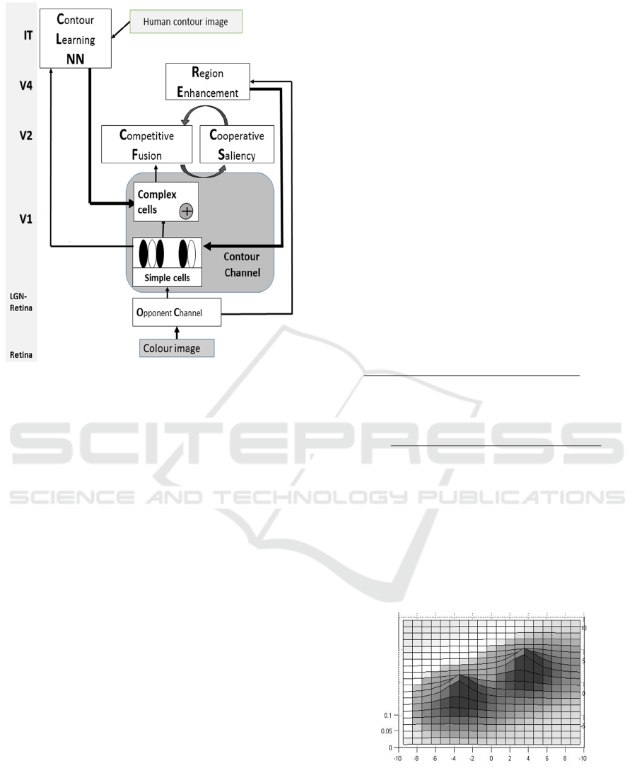
Figure 1: Scheme of the L-PREEN architecture.
2.1 Contour Channel Stage
The CC stage in L-PREEN models the behavior of the
simple and complex cells in V1. The activity of
simple cells is obtained through Gabor filters,
,,
()
,
for three scales (s=0,1,2), six orientations (k=0,…,5
corresponding to θ=0º, 30º, 60º, 90º, 120º, 150º),
deviations =1.0,2.0,4.0 and frequencies =
0.1,0.07,0.03.
The model equation for RG channel is detailed in
(1).
(
(
)
,
(
)
)=
()
⨂
,,
()
(1)
where, ⨂represents matrix convolution.
The complex cells in L-PREEN receive inputs
from the bottom-up pathway (BU) coming from the
OC stage and the top-down pathways (TD) of the RE-
V4 stage and the LCNN stage (see Figure 1). These
inputs are fused together following equation (2) with
=max(,0) and gain constants α, β and κ (1.0,
1.0, 0.6);
(
)
=∝
(
)
+
(
)
+
(
)
+
(
)
+
(2)
(
)
+
(
)
)
2.2 Competitive-Cooperative Loop
The inner BU-TD interaction is performed in the
competitive CF and cooperative CS stages through a
multiplicative competitive network with double
inhibition among spatial positions and among
orientations. This recurrent interaction detects,
regulates, and completes boundaries into globally
consistent contrast positions and orientations, while it
suppresses activations from redundant and less
important contours, thus eliminating image noise.
The CF activity,
()
, follows equation (3) with,
()
and
()
are Gaussian functions and
()
=
0.4,0.8,1.0
,
()
=
()
+
()
is the fusion
between the BU signal from the CC stage (
()
) and
the TD signal from the CS stage (
()
, see equation
4). [c]=max(c, 0), A4=10.0, Kh=1.0, Kf=5.0, Cc=0.3
and Ci=0.1.
(
)
=
()
−
∑∑
()
()
−
∑
()
()
+
()
+
∑∑
()
()
+
∑
()
()
(3)
()( )
()( )
() () () ()
()
() () () ()
5
ss s s
pqk pqk pqk pqk
s
ijk
ss s s
pqk pqk pqk pqk
zPUzNU
F
APU NU
=
+
∑
∑
∑∑
(4)
where
()
and
()
are the receptive field
lobules with bipole profile (see Figure 2), A
5
=0.001
is a constant and z(s) =max(s-α, 0), α=0.1.
This competition-cooperation recurrence is
computed in an iterative way following equations (3)
and (4). In our test simulations, convergence is
accomplished after 56 iterations.
Figure 2: Profile of the dipole.
2.3 Region Enhancement Stage
Region enhancement performs diffusion processes
from three channels.
SIGMAP 2016 - International Conference on Signal Processing and Multimedia Applications
90
These diffusions yield a colour coherent
homogenization within significant regions of the
natural scene. This region enhancement corresponds
to the surface perception.
For the diffusion process an iterative scheme
based in equation (5) is proposed. In this equation,
()
is the γ-channel diffusion, A7 =1.0 is a constant,
()
represents the OC signal rg, and
are the
nearest neighbors to position (i, j),
=
(
(
)
(
)
)
is the permeability with
()
=
∑
()
, Ke=1.0, Kp=10.0 are positive constants.
()
=
()
in =0
()
=
()
+
∑
()
,∈
+
∑
,∈
(5)
Fig. 4 shows L-PREEN diffusion outputs. These
diffusions (surface perception) will be filtered to
extract the contours which will behave as feedback.
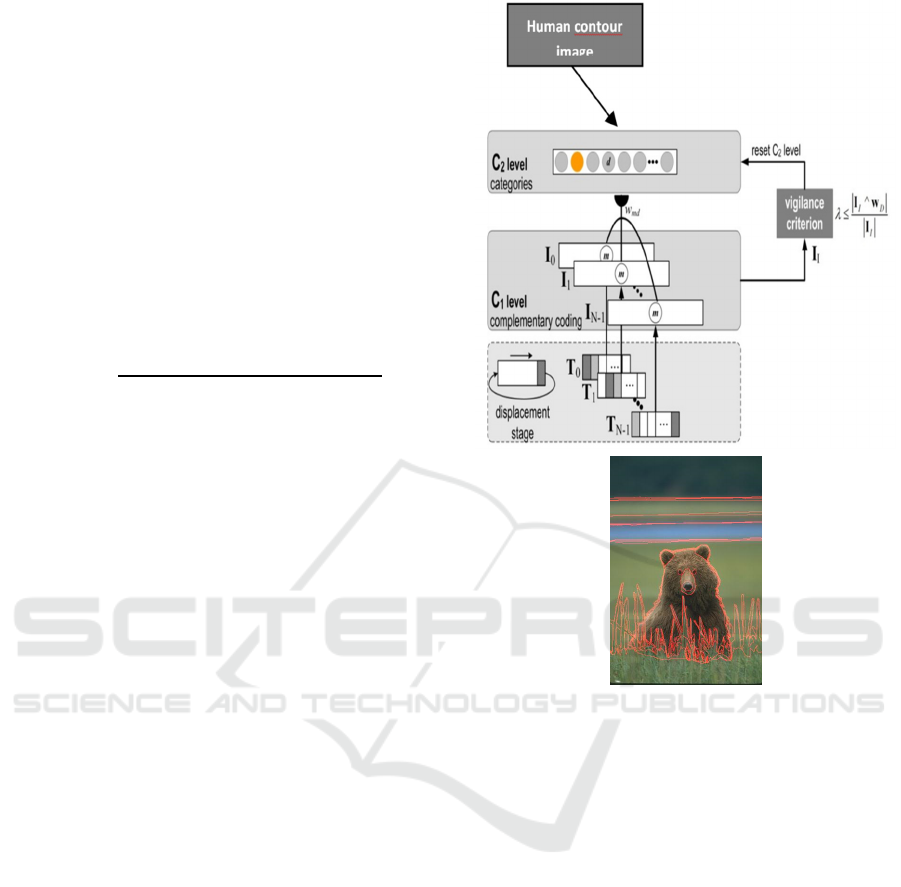
2.4 Contour Learning Neural Network
The CLNN stage includes a SOON neural network
(Antón et a., 2009) based in Fuzzy ARTMAP
(Carpenter et al., 1992) that merges the contour
information coming from different scales, in order to
generate the learning of the ground truth contours
traced by humans (see Figure 3-down).
The contour activity pattern Rij is expressed
following equation (6).
=(
(
)
,
(
)
,
(
)
,
(
)
,..,
(
)
,…,
(
)
,…, (6)
(
)
,
(
)
,
(
)
,
(
)
,..,
(
)
,…,
(
)
,…,
(
)
,…)
where (i, j) is the position, (
(
)
,
(
)
) is the pair
corresponding to the real and imaginary parts of the
Gabor filtering (see equation 1). SOON network has
two levels of neural layers, the input level C1 with 6
layers and complementary coding, and the
categorization level C2 (see figure 3-up). To link
these two levels, there is an adaptive filter with
weights
where prototypes learnt of the categories
generated are stored.
In the train phase, the positions belonging to
human contours of the ground truth images are taken
as a reference for contour pattern learning (see Fig. 3-
down). In the test mode, the weights of the selected
node,
(D=winner category) determine the
Figure 3: Up: Scheme of the SOON architecture. Down:
Original image with overlapped human contours. The
points of ground truth represented in red are the learning
points.
feedback signals of the LCNN contour learning stage
(
(
)
,
(
)
) (see equation (2)).
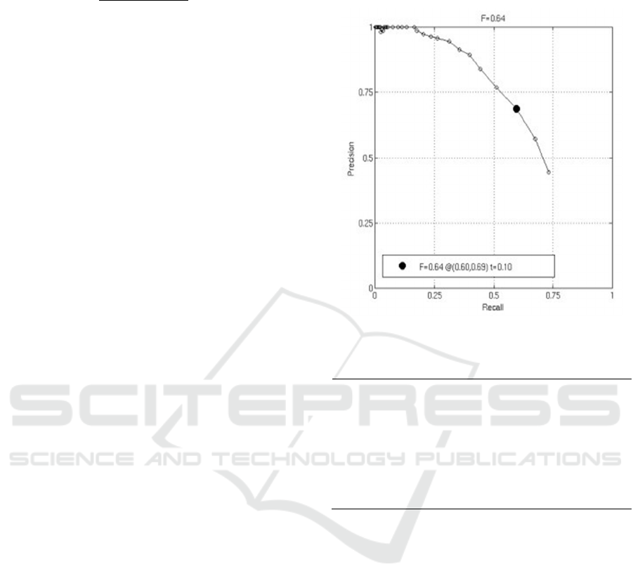
2.5 Experimental Results
We have used every single image of the BSD300
from the Berkeley Segmentation Dataset (Martin et
al., 2001), the 200 images for train and the 100 images
for test, together with their human segmented images
counterparts. The latter were taken as the ground truth
for learning process and to accomplish F-values. The
F-value is the harmonic mean of precision (the
fraction of true positives) and recall (the fraction of
ground-truth boundary pixels detected), at the optimal
detector threshold. Depending on the relative cost
between these measures, the F-value is expressed
according to Eq. (7) where P stands for precision, R
for recall and α is the relative cost.
Contour Learning and Diffusive Processes for Colour Perception
91
=
+
(
1−
)
(7)
For the tests performed using L-PREEN we chose
a relative cost α = 0.5,
The average F-value obtained is F=0.64 (0.60,
0.69), as showed in Fig. 4. Fig. 5 shows some of the
segmentation results obtained using L-PREEN We
are going to compare the L-PREEN results with a
method for boundary detection based in tensor voting
with perceptual grouping in natural scenes that has
been made available publicly. Perceptual groupings
achieve to extract illusory figures o completed
boundaries following the Gestalt visual perception
principles. Therefore, the comparison method
proposes a non-neural scheme of perceptual
groupings of natural figures in cluttered backgrounds
different from L-PREEN. Loss et al. (Loss et al.,
2009) proposed an iterative method based in
multiscale tensor voting. Loss et al.’s approach
consists in iterative removing image segments and
applying a new voting over the rest of the segments,
in order to estimate the most reliable saliency. The
tensor representation chosen was subsets of pixels to
form the tensor with ball or stick tensors initialization.
The decision on this representation is based in
reducing the number of tensors, what at the end
reduces the computation time. In this work they
present an evaluation of their method using two
datasets: fruit synthetic images and the BSDS300
Berkeley dataset. In the latter evaluation, they use
five base segmentation methods (Gradient Magnitude
(GM), Multi-scale Gradient Magnitude (MGM),
Texture Gradient (TG), Brightness Gradient (BG) and
Brightness/Texture Gradient (BTG), to generate a
Boundary Posterior Probability map (`segmentation
feeders’). This map is employed as a preprocessing
step for their method. In order to quantify the results,
they obtained the F-value and Precision-Recall
graphs. The F-values obtained using the five methods
over the 100 test images of the Berkeley Dataset
where 0.57, 0.58, 0.57, 0.60 and 0.62 respectively. L-
PREEN obtains an F-value of 0.64, as it is showed in
Table 1, which is a better result than all the five
versions of the comparison method.
We took the Matlab code of the gPb method
(Global Probability of Boundary) (Arbelaez et al.,
2011), third position in the ranking published in the
Berkeley-Benchmark http://www.eecs.berkeley.edu/
Research/Projects/CS/vision/bsds/bench/html/image
s.html) offered by their authors in the University of
Berkeley website and performed some executions for
the 100 test images, obtaining an average execution
time of 403.29 s per image, while L-PREEN needs
159.12 s.
Figure 4: Precision-recall curve.
Table 1: Comparative results.
Method F-value
Loss et al’s method with GM method 0.57
Loss et al’s method with MGM
method
0.58
Loss et al’s method with TG method 0.57
Loss et al’s method with BG method 0.60
Loss et al’s method with BTG method 0.62
L-PREEN 0,64
3 CONCLUSIONS
This work presents a new model, L-PREEN, for
detecting the boundaries and the surface perception of
colour natural images. This model is bio-inspired on
processes in V1, V2, V4 and IT visual areas of the
Human Visual System.
L-PREEN model includes orientational filtering,
competition among orientations and positions, and
cooperation through bipole profile fields and contour
learning. The proposed architecture has been
compared with Loss et al.’s method (Loss et al.,
2009), obtaining better results. A major advantage of
the L-PREEN model is its speed when compared to
other methods. L-PREEN can be implemented using
matrix and convolution operations, making it
compatible and scalable with parallel processing
hardware. This research will be our future work.
SIGMAP 2016 - International Conference on Signal Processing and Multimedia Applications
92
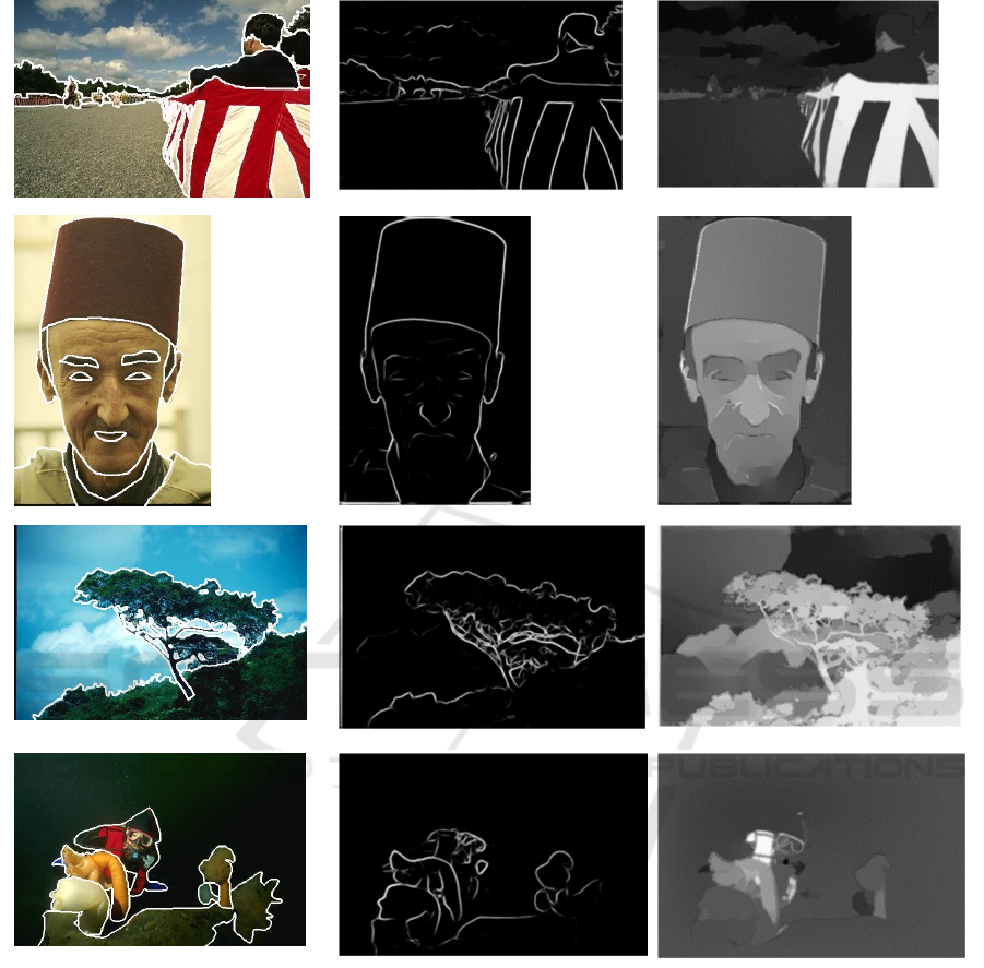
Figure 5: Examples of processing results using L-PREEN. Left column: original image with overlapped human contours.
Second column: L-PREEN boundary output. Third column: diffusion output (rg channel).
REFERENCES
Antón-Rodríguez, M., Díaz-Pernas, F. J., Díez-Higuera, J.
F., Martínez-Zarzuela, M., González-Ortega, D.,Boto-
Giralda, D., (2009). Recognition of coloured and
textured images through a multi-scale neural
architecture with orientational filtering and chromatic
diffusion. Neurocomputing, 72:3713–3725.
Arbelaez, P., Maire, M., Fowlkes, C. and Malik, J. (2011).
Contour Detection and Hierarchical Image
Segmentation. IEEE TPAMI, Vol. 33, No. 5, pp. 898-
916.
Carpenter, G.A., Grossberg, S., Markuzon, N., Reynolds,
J.H., Rosen, D.B., (1992). Fuzzy ARTMAP: A Aneural
Network Architecture for Incremental Supervised
Learning of Analog Multidimensional Maps. IEEE
Transactions on Neural networks, 3(5):698-712.
Grossberg, S., Williamson, J.R., (1999). A self-organizing
neural system for leaning to recognize textured scenes.
Vision Research, 39:1385-1406.
Grossberg, S., Huang, T.. (2009). ARTSCENE: A neural
system for natural scene classification. Journal of
Vision, 9(4):1–19.
Contour Learning and Diffusive Processes for Colour Perception
93

Hong, S., Grossberg, S.. (2004). A neuromorphic model for
achromatic and chromatic surface representaction of
natural images. Neural Networks, 17:787-808.
Kokkinos, I., Deriche, R., Faugeras, O., Maragos, P..
(2008). Computational analysis and learning for a
biologically motivated model of boundary detection.
Neurocomputing, 71(10-12):1798-1812.
Loss, L., Bebis, G., Nicolescu, M., Skurikhin, A.. (2009).
An iterative multi-scale tensor voting scheme for
perceptual grouping of natural shapes in cluttered
backgrounds. Computer Vision and Image
Understanding 113:126–149.
Martin, D., Fowlkes, C., Tal, D., Malik, J.. (2001). A
Database of Human Segmented Natural Images and its
Application to Evaluating Segmentation Algorithms
and Measuring Ecological Statistics. Proc. 8th Int'l
Conf. Computer Vision, 2: 416-423.
Mingolla, E., Ross, W., Grossberg, S., (1999). A neural
network for enhancing boundaries and surfaces in
synthetic aperture radar images. Neural Networks,
12:499-511.
Vonikakis, V., Gasteratos, A., Andreadis, I.. (2006).
Extraction of Salient Contours in Color Images. 4th
Panhellenic Conference of Artificial Intelligence
(SETN 2006), Lecture Notes in Computer Science,
3955:400-410, Heraklion, Greece.
SIGMAP 2016 - International Conference on Signal Processing and Multimedia Applications
94
