Calculation of Optimal Luminaires for Architectural Design
Rodrigo Leira
1
, Eduardo Fern
´
andez
1
and Gonzalo Besuievsky
2
1
Centro de C
´
alculo, Universidad de la Rep
´
ublica, Montevideo, Uruguay
2
Geometry and Graphics Group, Universitat de Girona, Girona, Spain
Keywords:
Inverse Lighting, Radiosity, Photometric Data, Luminaires.
Abstract:
The selection and location of optimal luminaries is a central aspect of architectural design. Its complexity
arises due to the diversity of existing luminaires, and the problems related to the need of achieving a set
of lighting goals and constraints. The use of computer simulation software can bring an improved support
in decision making at design time. CAD applications for illumination assessment are generally based on a
working forward strategy, where the designer selects all the design elements, in order to calculate the resulting
illumination. In this paper we present an inverse approach for the selection of luminaires, where the designer
defines a set of lighting intentions to satisfy, and then an optimization algorithm iterates, converging to a
feasible and optimal solution. The method allows to use a database consisting of hundreds of luminaires and
a set of possible locations. In each iteration, after the first reflection of a potential configuration is calculated,
the radiosity method is used to compute the final illumination of the scene.
1 INTRODUCTION
The selection and the location of luminaires are im-
portant steps in the process of architectural design. Its
complexity arises from the need of satisfying a set of
goals and constraints to ensure the efficiency, appeal,
and functionality aspects of the resulting environ-
ment. These set of constraints and goals are defined as
Lighting Intentions (LIs) (Russell, 2012). The prob-
lem of finding the illumination settings from LIs is
known as inverse lighting problem (ILP) (Marschner,
1998). Given its multiple factors, the designer must
adjust each of the variables involved with the aim of
satisfying the LIs. This is not a new dilemma and
existing professional illumination CAD tools, as for
example Dialux (DIALux, 2016), provide tools that
can serve this meaning. The main deficiency of these
is that they are based on a forward strategy that it is
not appropriate for optimization. Because of this, a
computer simulation module that is able to compute
optimal solutions, can provide great support.
We present a novel optimization method for ILP
that considers the position and main luminaire char-
acteristics (spatial and power distribution), to find the
optima for a given set of LIs. The method is based
on a low-rank approximation of the radiosity matrix
(Fern
´
andez, 2009) and the search of the optima by
means of the VNS (Variable Neighborhood Search)
meta-heuristic (Mladenovi
´
c and Hansen, 1997).
This paper proposes a technique that allows con-
sidering the way different types of luminaires emit
light, in the optimization process. The data of lu-
minaires is taken from databases provided by man-
ufacturers and is used to produce the first light reflec-
tion on the scene. Then, the low-rank radiosity (LRR)
method is used as an efficient engine to calculate the
final radiosity.
2 RELATED WORK
The technique presented deals with an inverse light-
ing problem that infers the properties of a physical
system from desired data. Inverse problems are ill-
posed and of interest in a wide range of fields in light-
ing engineering and lighting design. We use the ra-
diosity computation with the goal of solving such in-
verse problems looking for a global illumination so-
lution. This is partially based on the work done in
(Fern
´
andez and Besuievsky, 2012), where the LRR
method is used to solve the inverse lighting problem.
In the context of luminaire optimizations, many
methods have been developed to optimize the position
of a set of luminaires in a scene in order to produce
an approximation to the optimal lighting design. In
(Shikder et al., 2010) a method is formulated for plac-
ing two fixed luminaires into two separated sets of po-
sitions. They consider the photometric values of the
Leira R., Fernà ˛andez E. and Besuievsky G.
Calculation of Optimal Luminaires for Architectural Design.
DOI: 10.5220/0006102702030211
In Proceedings of the 12th International Joint Conference on Computer Vision, Imaging and Computer Graphics Theory and Applications (VISIGRAPP 2017), pages 203-211
ISBN: 978-989-758-224-0
Copyright
c
 2017 by SCITEPRESS – Science and Technology Publications, Lda. All rights reserved
203

luminaire but use two fixed luminaires that can be po-
sitioned on two disjoint set of points and optimize its
positioning. Other approach, similar to the previous
method, is introduced in (Uygun et al., 2015) for op-
timizing a set of luminaire positions. They also con-
sider the luminaire photometric data but without any
optimization performance. An interesting method is
presented for designing exterior lighting for building
in (Schwarz and Wonka, 2014) where they optimize
position, rotation and luminaire distribution but only
consider direct illumination and a reduced database of
luminaires.
2.1 Photometric Files and Polar Curves
of Luminaires
The presented approach focuses on calculating a first
reflection of the light emmited by the luminaire into
the geometry of the scene. That first reflection is then
used as the emission on the radiosity method. In or-
der to map the first reflection into the scene the po-
lar curve is used. The polar curves are taken from
photometric files, which are defined with the LM-63-
02 IESNA standard (IESNA-Computer-Committee,
1995) or its equivalent EULUMDAT format. Data
from these files have to be transformed to represent
the incident luminous flux (measured in lumens) re-
cieved by a given patch in the scene. In this report we
use a database composed of 1516 luminaires extracted
from (Philips, 2016) and (Cree, 2016).
2.2 LRR
The method presented assumes that all surfaces in the
scenes are Lambertian reflectors. This assumption al-
lows to speed up the calculations, evaluating thou-
sands of luminaires configurations in a short time.
Our solver is based on the radiosity problem, taking as
emission the first reflection calculated using the polar
curves.
The discrete radiosity equation is formulated as:
(I − RF)B = E (1)
where E is a vector containing the light emissions for
each patch in the scene, I is the identity matrix, R is a
diagonal matrix containing the diffuse reflectivity for
each patch. F is a matrix containing the form factors,
where F(i, j) is a value between 0 and 1 indicating the
proportion of the total light radiated by the patch i go-
ing to patch j. B is a vector containing the radiosity
values to be found (Cohen et al., 1993). LRR takes
into consideration the low-rank properties of the RF
matrices (Fern
´
andez, 2009). RF size is O(n
2
) but due
to the spatial coherence of the radiosity values, i.e.
close patches typically have similar radiosity values,
RF can be approximated by the product UV
T
where
U and V are n × k matrices that can be computed ap-
plying O(n
2
) operations, where n  k. Further, U is a
dense matrix and V is a sparse matrix. In addition to
the previous approximation, the Sherman-Morrison-
Woodbury (Golub and Van Loan, 2013) formula is
used to calculate an approximation of the inverse of
the radiosity matrix M:
M = (I − RF)
−1
≈ (I +YV
T
) =
˜
M (2)
where Y = U(I − V
T
U)
−1
Then we can reduce Eq. (1) to the following
matrix-vector product:
˜
B =
˜
ME, which can be also
formulated as:
˜
B = E +Y(V
T
E) (3)
In this equation,
˜
B is an approximation of B. This final
reduction grants the ability of calculating
˜
B in O(nk)
operations and consuming O(nk) memory. The ben-
efits of this are straightforward, on the condition that
the scene geometry does not change. This method can
be used to solve inverse lighting problems, gaining a
speed up over traditional radiosity methods, allowing
us to calculate the radiosity of static scenes contain-
ing thousands of elements, and allowing the chang-
ing of the emitters. Like this, other methods have
been proposed to speed up the calculations of Y and
V (Aguerre and Fern
´
andez, 2016).
2.3 Optimization Problem
The ILP is determined as the process of placing the
emitters in order to achieve a set of Lighting Inten-
sions. This process was proposed as an alternative to
solving Eq. (1), which results in an ill-posed linear
system because of the low-rank properties of the RF
matrix (Fern
´
andez and Besuievsky, 2015).
VNS is the method used for seeking for optimal
configurations. The main idea of VNS is the succes-
sive exploration of neighborhoods (usually nested),
where a finite and random set of representatives is
selected with the intention of finding a solution that
is better than the best found on previous iterations.
What is interesting about this method is that it walks
from neighborhood to neighborhood in a systematic
fashion in order to escape from local optima, and
therefore improving odds of finding the global optima
(Talbi, 2009).
2.4 Hemi-cube
The presented approach uses a hemi-cube to calcu-
late the emission from a luminaire into the scene. The
GRAPP 2017 - International Conference on Computer Graphics Theory and Applications
204

hemi-cube method used is based on the concept first
introduced by (Cohen and Greenberg, 1985). On Co-
hen proposal the hemi-cube consists of 5 projections,
or faces, divided into many pixels where the patches
of the scene are projected. For each pixel the ∆F
is calculated as viewed from the center of the patch
where the hemi-cube is positioned. Given the hemi-
cube centered on the barycenter of patch i, onto which
a patch j is projected, the sum of the ∆F (form fac-
tors) associated to patch j is F(i, j). This summation
is performed for each patch obtaining a vector with
all form-factors for the scene for the hemi-cube posi-
tioned at patch i. When many patches of the scene are
projected onto the same pixel of the hemi-cube, the
patch seen in that pixel is determined by calculating
the distance to patch i and selecting the nearest. We
use a variation of the form factors where each pixel
is associated to its delta solid angle (∆Ω), see Section
3.3. This information can be used altogether with the
information taken from photometric files to build the
first reflection of the light in the scene.
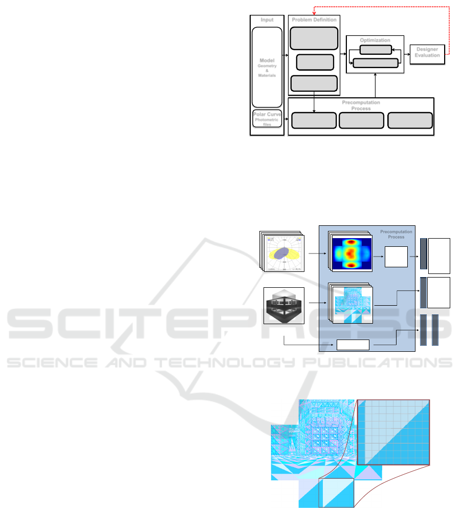
3 METHOD OVERVIEW
The pipeline design of the proposed approach is de-
scribed in Fig. 1. It starts from a given architectural
interior model for lighting design with reflectance
surfaces already defined. Then the user configures
the parameters to specify the zones where the light
sources can be placed as well as the variables to op-
timize. This includes the geometric restrictions and
other lighting intentions to achieve, as for instance,
the goals and constraints related to energy consump-
tion, with the aim of finding the optimal solution.
Also the database containing the desired set of lu-
minaries is provided. Then the precomputation pro-
cess provides the hemi-cubes needed for the optimiza-
tion as well as the matrices obtained from the LRR
method. Next, the optimization process is executed to
find a candidate configuration, which is evaluated by
the designer. Regarding the resulting values, the de-
signer can modify the setting parameters in order to
search for a new solution.
3.1 Precomputation
Before the optimization process begins, a precompu-
tation process is executed (see Fig. 2). A compact
representation of the scene information is obtained by
means of the LRR method. Also, the database with
the photometric files is preprocessed in order to cre-
ate the hemi-cube L associated to each polar curve.
Next, the process of creating each hemi-cube view H
Evaluation
Radiosity solver
Designer
Evaluation
Problem Definition
Model
Geometry
&
Materials
Optimization
Light Intentions:
Global Illumination,
Emitters
Filters
Optimization
Variables
Polar Curve
Photometric
files
Input
Precomputation
Process
Low-rank Radiosity
Hemi-cube calculation
from luminaries
ubication.
Transform Polar
Curves into hemi-
cubes. Sort.
Ubication of
luminaries
Figure 1: Pipeline system.
for the scene from each possible luminaire location
is performed. These hemi-cubes are calculated using
the z-buffer technique and a color based encoding for
the patch indexes (see Fig. 3). Both L and H are rep-
resented as matrices.
Polar Curves
Polar Curves Database.
Geometric Model
of the scene
Views of the scene
one hemi-cube H for each
element on the source surface
Transformed Polar Curve
to an hemi-cube L
View Hemi-
cubes
Hemi-cube
with patches
visible for
each pixel
Y & V
calculation
Y
V
Precomputation
Process
Polar Curve
Hemi-cubes
Hemi-cube
with
lumens
emited to
each pixel
Sort
Order hemi-
cubes by
similarity
Figure 2: Precomputation process. Hemi-cubes L’s and H’s
are generated, as well as Y and V matrices. L’s are sorted
(Algorithm 1).
15 15 15 15
15
15 15
15
15
15 15
15
15 15
15
15 15
15
15 15
15
15
15
15 15
15
15
15 15
15
15 15
15
15
15
15
15
15
33 33 33 33 33
33
33
33 33
33 33 33 33 33
33
33
33
33 33 33 33 33
33
33
33 33 33 33 33
33
33
33 33 33 33
33 33 33 33
33 33
33
11
11
11
11
11
11
11
11
45
15
Figure 3: Hemi-cube view of the scene H. The colors en-
code the index for each patch. In the top-right, the index
associated to each pixel is displayed.
The proposed method uses the VNS meta-
heuristic, therefore, we need to sort the L’s and H’s
hemi-cubes in a way that allows to build the neighbor-
hoods. For the H’s views, the neighborhoods are built
using their positions. The neighbors of an location are
those positions that are close in space. On the other
hand, to calculate the neighborhoods for the hemi-
cubes based on polar curves, we use the Euclidean
Calculation of Optimal Luminaires for Architectural Design
205

distance (Frobenius norm) to sort them by means of
Algorithm 1.
Algorithm 1: Sort luminaires hemi-cubes.
Require: D #
D is a n×n distance matrix
1: I ← [1:n]
2: for k=1:n-1 do
3: subD
k
←D(1:k,k+1:n)
4: (min,i, j) ← minimum(subD)
5: if min < δ then
6: D ← moveCol(D, j, i)
7: D ← moveRow(D, j, i)
8: I ← move(I, j, i)
9: else
10: D ← moveCol(D, j, k)
11: D ← moveRow(D, j, k)
12: I ← move(I, j, k)
13: end if
14: end for
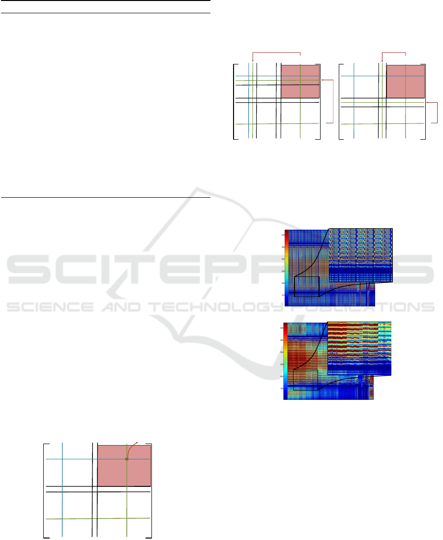
15: return I
The sorting algorithm receives a matrix D as in-
put, where D(i, j)=||L
i
−L
j
||
Fr
, is the Euclidean dis-
tance between the hemi-cubes of luminaires i and j.
In the k
th
step, I(1:k) is a list of sorted luminaires, and
I(k+1:n) is the remaining set of unsorted luminaires.
When adding a new luminaire to the sorted list, an
unsorted luminaire j is chosen such that it minimizes
the distance to any luminaire in the sorted list. To do
so, the first step (line 3) takes the matrix subD
k
that
contains all the distances between both sets. Then the
luminaires i and j are selected such that i belongs to
the sorted list and j to the unsorted set, and its Eu-
clidean distance is minimal (line 4 and Fig. 4). If that
distance is less than a predefined threshold δ, then lu-
minaire j is placed in the sorted list between the lumi-
naires i and i+1 (lines 6 to 8 and Fig. 5 (a)), otherwise
it is located at the end of the sorted list (lines 10 to 12
and Fig. 5 (b)). The algorithm starts including one
luminaire in the sorted list, and at each step a new el-
j
j
i
k+1
k+1
k
⋯
k
⋯
⋯
⋯
i
minimum(subD
𝑘
)
subD
𝑘
Figure 4: subD
k
contains the distances between the sorted
and unordered luminaires. subD
k
(i, j) contains the mini-
mum distance between them. The minimum value on the
sub-matrix is selected.
ement is added to it. For the unsorted set the opposite
happens. It starts with all the luminaires but the one
selected, and at each step one element is extracted. At
the end, all the luminaires belong to the sorted list.
Finally the algorithm returns a vector with the sorted
indexes (line 15). In this vector, the position i contains
the index of the i
th
luminaire in the sorted list.
j
j
i
i+1
i+1
k+1
k
⋯
⋯
⋯
⋯
i
subD
𝑘
k+1
k
(a) min < δ
j
j
i
k+1
k
⋯
k
⋯
⋯
⋯
i
subD
𝑘
k+1
(b) min ≥ δ
Figure 5: Sorting steps. Relocation of i row and j column.
An example with the result of sorting the selected
luminaires (Sec. 2.1) can be seen in Fig. 6. It can
be observed that a greater similarity exists between
consecutive columns on the sorted list.
lm
(a) Unsorted luminaires
lm
(b) Sorted luminaires
Figure 6: Plot of the database containing the luminaire
hemi-cubes. In the image, each column represents a hemi-
cube (reshaped as a vector).
3.2 Optimization
The optimization process (see Fig. 1) initializes the
set of variables using a random seed. Using VNS
we search for variables in the same neighborhood to
the ones selected, using the positions and the list of
sorted luminaires calculated on the precomputation
process. In each step, the hemi-cubes H
i
and L
l
of
a selected view i and a luminaire l are combined to
calculate the lumens received for each patch as the
GRAPP 2017 - International Conference on Computer Graphics Theory and Applications
206

first reflection. The luminous emittance is then cal-
culated, using the direct luminous emittance (first re-
flection) as the emission on the radiosity equation (see
Eqs. (1) and (3)). After that, the illumination is com-
pared to the best solution found, following the VNS
meta-heuristic.
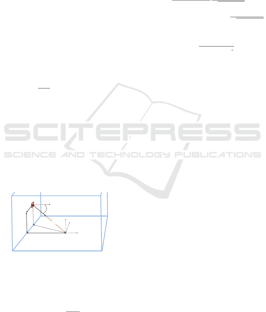
3.3 Direct Luminous Emittance
Calculation
In this section we focus on achieving a first reflection
that is used as emission in the radiosity equation. In
order to construct it, we use the hemi-cube technique
in conjunction with the information contained in the
photometric files.
Eq. (4) shows how to obtain the direct luminous
emittance E
i,l
(p) of each patch p on the scene, given
a luminaire l positioned at patch i:
E
i,l
(p) =
R(p)
A(p)
∑
{(u,v):
H
i
(u,v)=p}
∆
∆
∆Ω
Ω
Ω(u,v)L
l
(u,v) (4)
where p is a patch on the scene, R(p) is its dif-
fuse reflectivity, A(p) is its area, H
i
is the hemi-cube
view of the scene (Fig. 3), in the matrix ∆
∆
∆Ω
Ω
Ω each of
its elements (u, v) contains the solid angle, measured
in sr, of pixel (u,v) (Fig. 7). L
l
(u,v) contains the
number of candelas transmitted through pixel (u,v)
by the luminaire l. L
l
(u,v) is built using the infor-
mation provided in polar curves, assigning the value
corresponding to the emission in candelas (lm/sr) of
the luminaire to each pixel. The patch seen through
each pixel on hemi-cube H
i
is determined using the
z-buffer algorithm.
Z
Y
X





z
y

1
(u,v)


Figure 7: ∆Ω calculation of pixel (u,v).
Each addend ∆
∆
∆Ω
Ω
Ω(u,v)L
l
(u,v) of Eq. (4) deter-
mines the luminous flux (i.e. the number of lumens)
that are transmitted through pixel (u,v) and the whole
sum is the incident luminous flux (lm) on patch p.
Each ∆
∆
∆Ω
Ω
Ω(u,v) is determined by Eq. (5):
∆
∆
∆Ω
Ω
Ω(u,v) =
4π∆A
A
s
ˆ
t · ˆn (5)
where ∆A is the area of pixel (u,v), A
s
is the area of
the sphere of radius r centered on point o (4πr
2
), ˆn
is a unit vector normal to the pixel, and
ˆ
t is a unit
vector centered on the pixel with a radial direction.
The scalar product
ˆ
t · ˆn determines the cosine of α.
Therefore Eq. (5) can be expressed as follows:
∆
∆
∆Ω
Ω
Ω(u,v) =
4π∆A
4π(x
2
+ y
2
+ z
2
)
1
p
x
2
+ y
2
+ z
2
(6)
because r
2
=x
2
+ y
2
+ z
2
, and
ˆ
t · ˆn =
1
p
x
2
+ y
2
+ z
2
resulting in Eq. (7):
∆
∆
∆Ω
Ω
Ω(u,v) =
∆A
(x
2
+ y
2
+ z
2
)
3
2
(7)
The sum of all ∆
∆
∆Ω
Ω
Ω(u,v) equals 2π. Finally, since
E
i,l
is the direct luminous emittance (lx), then the in-
cident luminous flux on patch p is divided by A(p)
(which determines the direct illuminance) and multi-
plied by reflectivity R(p).
4 IMPLEMENTATION
In order to reduce the resources needed for our
method, or to achieve better results in some cases, we
use the following implementation strategies:
Tabu Search: We use the Tabu Search method to
discourage the coming back to previously-visited so-
lutions (Glover and Laguna, 1997).
Empty Luminaire: Since we are optimizing the
configuration of luminaires it seems to be a good idea
to introduce the concept of an empty luminaire. This
luminaire emits no light and is used to relax the num-
ber of luminaires marked by the designer. In this way
the optimization process is allowed to use empty lu-
minaires that consumes 0 watts, so that it is possible
to achieve configurations with less luminaires. This is
performed by adding a hemi-cube L
0
filled with zeros
(no emission).
Probability of Change for Variables: We use three
variables to configure a luminaire, one for the lumi-
naire index and two for its location. When searching
for a candidate within the current VNS neighborhood,
the neighborhood establishes the number of variables
that can be changed at the same time. Since the car-
dinality for the domain of each of these variables is
different, a higher chance of change is given to the
variable of larger cardinality.
Polar Curve Hemi-cube: We focus on calculating
the emission for the lower half space only. This is
implemented with the hemi-cube L.
Calculation of Optimal Luminaires for Architectural Design
207

5 EXPERIMENTS AND RESULTS
Different experiments are performed in the literature
(Shikder et al., 2010; Uygun et al., 2015; Fern
´
andez
and Besuievsky, 2014) to validate their particular re-
sults. The experiments chosen are used to satisfy
some useful lighting standards, as well as to consider
realistic objectives and constraints for design. In all
experiments performed in this section, the luminaires
are placed on the roof of a patio scene (see Fig. 8)
The target surface for measuring light uniformity (for
Section 5.2) and power efficiency (for Section 5.3),
are the patches that defines the floor of the patio. All
experiments use a database consisting of 1517 hemi-
cubes L (1516 generated from the photometric files
and the hemi-cube related to the empty luminaire L
0
)
is used along with a scene consisting of 21824 trian-
gles. All instances were executed 30 times (indepen-
dent runs) and all optimizations perform a maximum
of 15000 radiosity calculations. The simulations were
conducted on a desktop computer, with Intel quad-
core i7 processor and 16 Gbytes of RAM. The code
was implemented mainly in MATLAB (MATLAB,
2014), also using C++ and OpenGL.
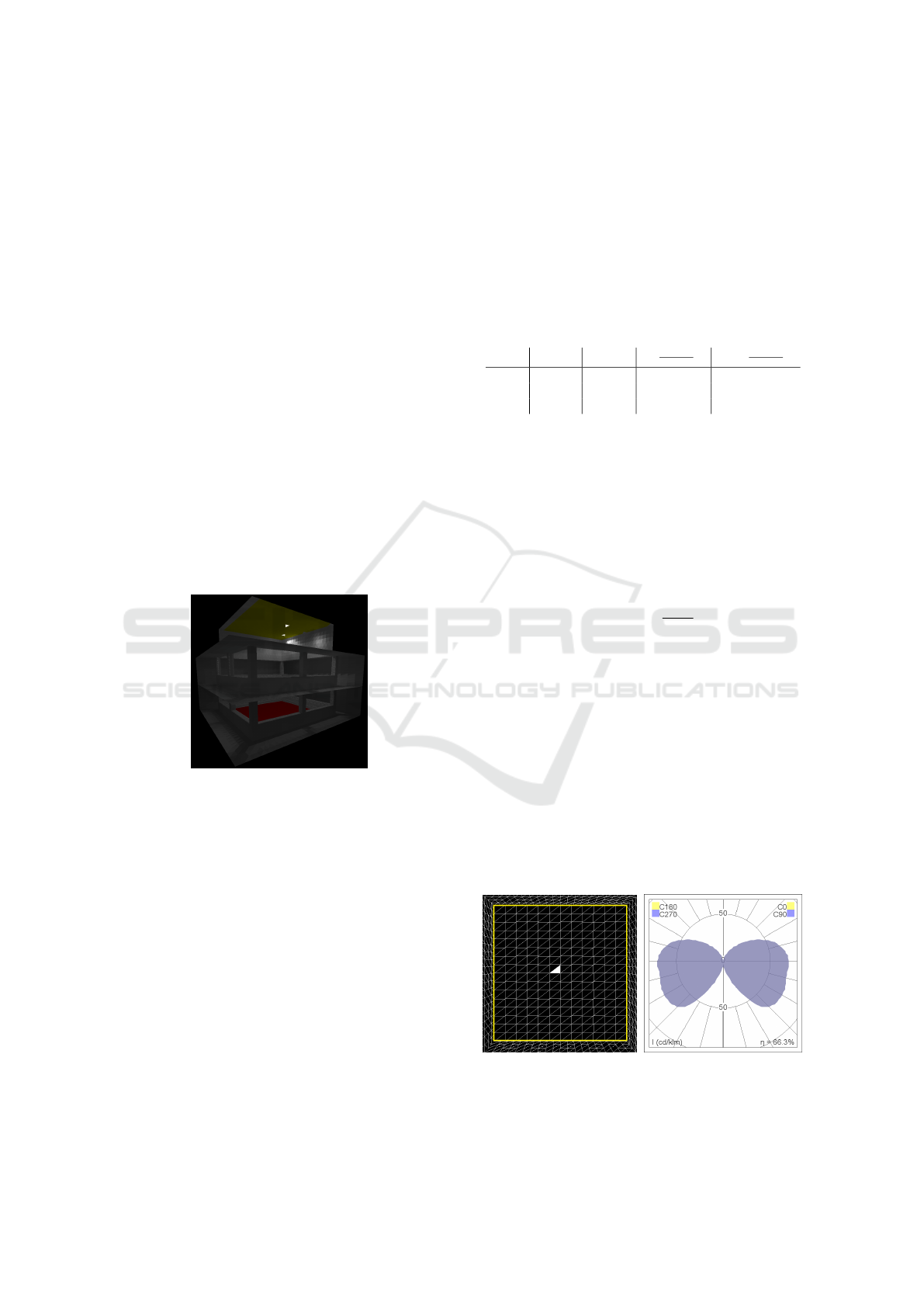
Figure 8: Lighting calculated for the scene. The possible
positions of luminaires are colored in yellow and the target
surface in red. White patches represent the places where the
two luminaires were placed in the rendered configuration.
5.1 Convergence
The first experiment is meant for analyzing the effec-
tiveness of the algorithm. Here we consider as op-
timization target the radiosity output
˜
B
T
, previously
calculated for a given configuration of luminaires and
positions. The objective is to minimize the Euclidean
distance between the radiosity
˜
B of the tested config-
urations and
˜
B
T
:
minimize : k
˜
B −
˜
B
T
k
2
(8)
The results for this experiment can be seen on Ta-
ble 1. It shows the number of runs in which the target
was found, the mean of the number of radiosity cal-
culations, the mean of the relative error, and the worst
relative error found. The algorithm stops when Eq. (8)
is 0. For the case of two luminaires, even though the
exact solution was found only one time, the mean and
worst relative errors show that the solutions are close
to the target. The use of three luminaires returned
similar results.
Table 1: Optimization results for minimizing the distance to
a given lighting.
# lum # found µ(#rad) µ

k
˜
B−
˜
B
T
k
2
k
˜
B
T
k
2

max

k
˜
B−
˜
B
T
k
2
k
˜
B
T
k
2

1 29 5139 3.0×10
−3
9.0×10
−2
2 1 14876 4.3×10
−2
6.0×10
−2
3 0 15000 3.1×10
−2
5.3×10
−2
5.2 Light Uniformity
The achievement of lighting uniformity is an impor-
tant goal to be considered in the design of lighting
systems (Staff et al., 2011). To obtain this goal,
the coefficient of variation (σ/µ) is minimized. This
coefficient is a normalized measure of dispersion
(Canavos, 1984).
minimize :
σ(
˜
B)
µ(
˜
B)
(9)
This experiment is performed using only one lu-
minaire. The expected result consists in finding a lu-
minaire centered on the roof, with a symmetric polar
curve that has greater light intensity on the angles that
point to the floor borders. The solutions found can be
seen in Fig. 9, where the position found for each so-
lution is centered on the roof (Fig. 9 (a)). The polar
curve (Fig. 9 (b)) is symmetric in all planes having
greater emission in the angles that are further from
the normal (illuminating patches that are more dis-
tant). The resulting lighting for the central patch and
the luminaire that was selected 29 times from Figs. 9
(a) and (b) respectively, can be seen in Fig. 10.
(a) Position selected on the
roof, on all runs, marked as
a white triangle.
(b) Polar curve found on 29
runs.
Figure 9: Results for optimizing the lighting uniformity.
GRAPP 2017 - International Conference on Computer Graphics Theory and Applications
208

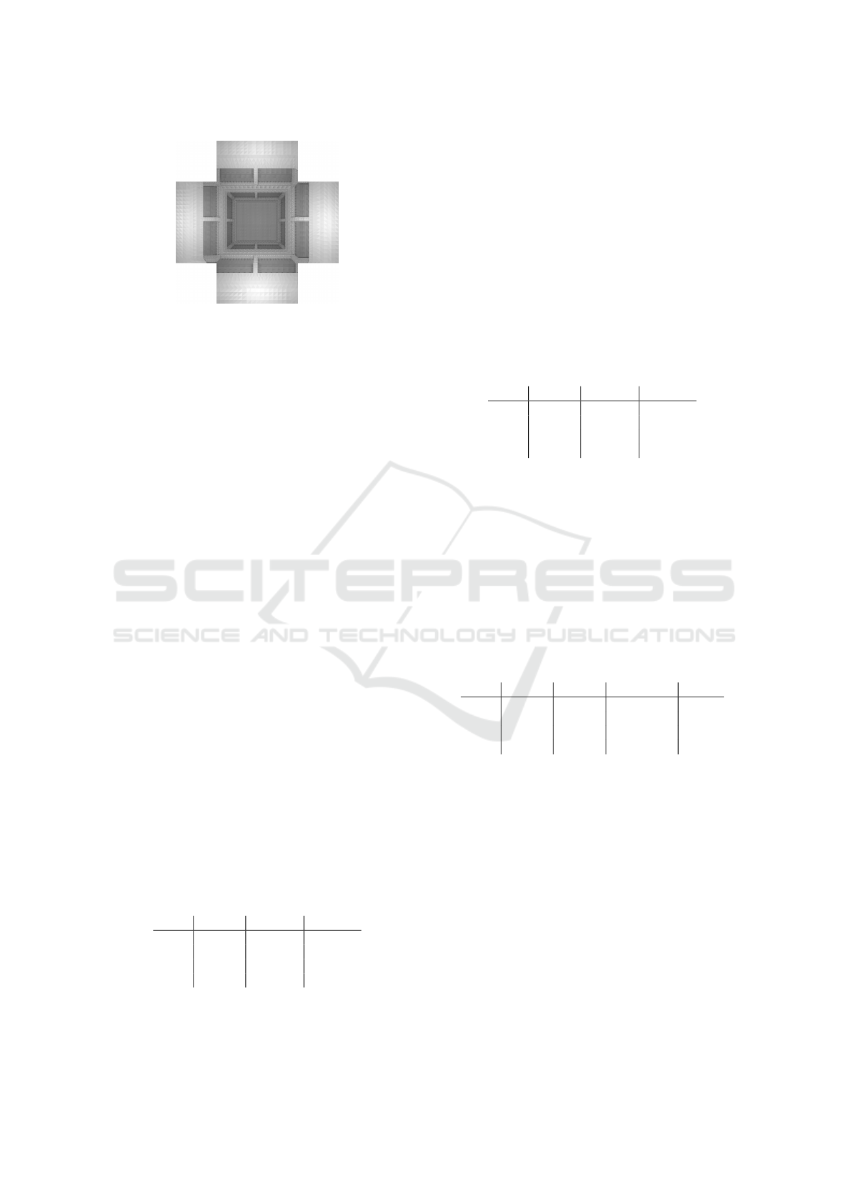
Figure 10: Hemi-cube view of the lighting result when op-
timizing the uniformity of the floor Section 5.2.
5.3 Power Efficiency
This experiment consists in minimizing the power
consumption for luminaires subject to certain illumi-
nance bounds in the target surface:
minimize :
n
∑
i=1
P
i
, i ∈ 1..n (10)
sub ject to :
(
min(I) >= 100lm
max(I) <= 750lm
where n is the number of luminaires placed in the
scene, P
i
is the power in watts consumed by the i
th
luminaire and I is a vector containing the illuminance
values found in each patch of the target surface. In
this test we start from a single luminaire and then we
do successive increments by one luminaire. The main
idea of this approach is to add new configurations to
the space of solutions, leading to better results. The
existence of the empty luminaire allows maintaining
the solutions of previously explored search spaces to
the new space of solutions. Therefore, the addition of
luminaires maintains the previous solutions and ex-
pands it to include new configurations.
When using a single luminaire, the best solution
found consumes 274 W. To validate this solution, we
evaluate each adjacent position with all the luminaires
of the database. To prove that, the solution found is
at least a local optimum. Next, the successive incre-
ments in the number of luminaires are executed and
improve the solution as expected, see Table 2.
Table 2: Optimization results for different number of lu-
minaires using hemi-cubes of size 512x512. The objective
consists in minimizing the power consumption.
# lum best (W) worst (W) µ ± σ (W)
1
(1)
274 431
(2)
379 ± 75
2 157 174 160± 4
3 138 173 154 ± 11
4 125 173 152 ± 10
1
Not all iterations ended with a valid configuration.
2
Maximum luminaire power is returned when no
valid solution was found.
5.4 Sorting Algorithm
All previous experiments were performed using the
sorted L’s hemi-cubes, by means of the algorithm in-
troduced in Algorithm 1. Here we perform the ex-
periment for optimizing the power efficiency (Sec-
tion 5.3) again but without applying the sorting al-
gorithm (using the database as seen in Fig. 5 (b)). Ta-
bles 2 and 3 show that the results without applying the
sorting algorithm are more power consuming than the
ones obtained when using the sorted database.
Table 3: Optimization results for different number of lumi-
naires using hemi-cubes of size 512x512 without sort. The
objective consists in minimizing the power consumption.
# lum best (W) worst (W) µ ± σ (W)
1 431 431 431± 0
2 371 442 433 ± 14
3 365 453 417 ± 30
4 365 454 430 ± 23
5.5 Performance
All optimizations performed in this section are based
on the same goals and constrains used in the power
efficiency experiment (Section 5.3).
Number of Luminaires: The relation between the
number of luminaires and the time needed for the op-
timization process is shown in Table 4, where there is
a rough linear relation between them.
Table 4: Optimization results using 512×512 hemi-cubes,
after 15000 radiosity calculations each.
# lum best (s) worst (s) µ ± σ (s) #rad/s
1 335 398 339 ± 12 44
2 566 717 578 ± 29 26
3 787 827 809 ± 9 19
4 1.0×10
3
1.2×10
3
1.1×10
3
± 12 14
Hemi-cube Size: Table 5 shows the power of the
solutions and timings for different hemi-cube sizes
and 4 luminaires. Smaller hemi-cubes results in larger
speedups but also in larger errors. This is due to the
fact that in general, smaller hemi-cubes contain less
accurate information about the scene.
For the precomputation step, an experiment was
conducted to measure its execution time for different
hemi-cube sizes. In Table 6, the size of the hemi-cube
is roughly proportional to the precomputation time.
6 CONCLUSIONS
A new technique is introduced for lighting opti-
mization considering hundreds of luminaires. The
Calculation of Optimal Luminaires for Architectural Design
209

Table 5: Optimization for 4 luminaires and different hemi-
cubes.
H µ±σ (W) µ±σ (s) error speedup
512 × 512 152±10 1061±12 - -
256 × 256 162±11 408±8 0.068 2.6
128 × 128 186±13 262±14 0.225 4.1
64 × 64 260±35 224±13 0.711 4.8
Table 6: Time results for the precomputation process.
H total time (s) speedup
512 × 512 20654 -
256 × 256 4860 4.3
128 × 128 1382 14.9
64 × 64 354 58.3
method is mainly based on the use of the hemi-
cube technique, the sorting of luminaires according
to their similarity, and the use of an optimization
meta-heuristic (VNS). The developed method allows
to evaluate thousands of configurations, with a set of
more than 1500 luminaires, in few minutes. The con-
vergence of the method was evaluated resulting in a
relative error up to 0.043. The relevance of the sorting
of luminaires was evaluated and proved to improve
the optimization. The technique performed well in
tests related to light uniformity and power efficiency.
The selection of the hemi-cube size should take into
consideration a trade off between the time of the al-
gorithm and the error of the results.
Further steps should include the exploration of
other techniques to perform the sorting of the lumi-
naire hemi-cubes, as well as the use of both (upper
and lower) hemi-cubes to model luminaire emission.
Also it is important to consider the orientation and tilt
of the luminaire as optimization variables, since polar
curves can be non-symmetrical and so studying fur-
ther techniques that allow to dynamically rotate the
polar curves (maintaining similar performance) is an
important step to follow. In order to consider non-
Lambertian surfaces it is necessary to explore new
rendering techniques that allow to maintain similar
performance. Finally, it would be useful to consider
the influence of daylighting in the optimization pro-
cess.
ACKNOWLEDGEMENTS
The work was supported by project
FSE 1 2014 1 102344 from Agencia Nacional
de Investigaci
´
on e Innovaci
´
on (ANII, Uruguay) and
project TIN2014-52211-C2-2-R from Ministerio de
Econom
´
ıa y Competitividad, Spain.
REFERENCES
Aguerre, J. P. and Fern
´
andez, E. (2016). A hierarchical fac-
torization method for efficient radiosity calculations.
Comput Graph, (to appear).
Canavos, G. (1984). Applied probability and statistical
methods:. Little, Brown.
Cohen, M. F. and Greenberg, D. P. (1985). The hemi-
cube: a radiosity solution for complex environments.
In SIGGRAPH Comput Graph 1985, pages 31–40.
Cohen, M. F., Wallace, J., and Hanrahan, P. (1993). Ra-
diosity and Realistic Image Synthesis. Academic Press
Professional, Inc., San Diego, CA, USA.
Cree (2016). Cree europe s.r.l a s.u., http://www.cree-
europe.com/en/doc-tecnica-dbf.php.
DIALux (2016). Dial. light building software. www.dial.de.
Fern
´
andez, E. (2009). Low-rank radiosity. In Proc.
Iberoamerican Symposium in Computer Graphics
(SIACG 2009), pages 55–62.
Fern
´
andez, E. and Besuievsky, G. (2012). Inverse lighting
design for interior buildings integrating natural and ar-
tificial sources. Comput Graph, 36(8):1096–1108.
Fern
´
andez, E. and Besuievsky, G. (2014). Efficient in-
verse lighting: A statistical approach. Autom Constr,
37(Complete):48–57.
Fern
´
andez, E. and Besuievsky, G. (2015). Inverse opening
design with anisotropic lighting incidence. Comput
Graph, 47(1):113–122.
Glover, F. and Laguna, M. (1997). Tabu Search. Kluwer
Academic Publishers, Norwell, MA, USA.
Golub, G. and Van Loan, C. (2013). Matrix Computations.
Johns Hopkins Studies in the Mathematical Sciences.
Johns Hopkins University Press.
IESNA-Computer-Committee (1995). IESNA standard file
format for electronic transfer of photometric data.
IESNA lighting measurements series. IESNA.
Marschner, S. R. (1998). Inverse Rendering for Com-
puter Graphics. PhD thesis, Ithaca, NY, USA.
AAI9839924.
MATLAB (2014). version 8.3.0 (R2014a). The MathWorks
Inc., Natick, Massachusetts.
Mladenovi
´
c, N. and Hansen, P. (1997). Variable neighbor-
hood search. Comput. Oper. Res., 24(11):1097–1100.
Philips (2016). Philips lighting holding b.v.,
http://www.lighting.philips.com/main/support/
support/dialux-and-other-downloads.html.
Russell, S. (2012). The Architecture of Light - Architectural
Lighting Design Concepts and Techniques. Concept-
nine.
Schwarz, M. and Wonka, P. (2014). Procedural design
of exterior lighting for buildings with complex con-
straints. ACM Trans. Graph., 33(5):166:1–166:16.
Shikder, S. H., Mourshed, M. M., and Price, A. D. F. (2010).
Luminaire position optimization using radiance based
simulation: a test case of a senior living room. In
Computing in Civil and Building Engineering.
Staff, B. S. I., Institution, B. S., and for Standardiza-
tion. CPL/34/10, E. C. (2011). Light and Lighting -
GRAPP 2017 - International Conference on Computer Graphics Theory and Applications
210

Lighting of Work Places: Indoor work places. Part 1.
BSI.
Talbi, E.-G. (2009). Metaheuristics: From Design to Imple-
mentation. Wiley Publishing.
Uygun, I., Kazanasmaz, Z., and Kale, S. (2015). Opti-
mization of energy efficient luminaire layout design
in workspaces. In Scartezzini, J.-L., editor, CISBAT
2015, pages 301–306, Lausanne. LESO-PB, EPFL.
Calculation of Optimal Luminaires for Architectural Design
211