Can a Driver Assistance System
Determine if a Driver is Perceiving a Pedestrian?
Consideration of the Driver’s Visual Adaptation to Illumination Change
Yuki Imaeda
1
, Takatsugu Hirayama
1
, Yasutomo Kawanishi
1
,
Daisuke Deguchi
2
, Ichiro Ide
1
and Hiroshi Murase
1
1
Graduate School of Information Science, Nagoya University, Furo-cho, Chikusa-ku, Nagoya-shi, Aichi, Japan
2
Information Strategy Office, Nagoya University, Furo-cho, Chikusa-ku, Nagoya-shi, Aichi, Japan
Keywords:
ITS, Driving Assistance, Detectability, Ambient Light, Visual Adaptation.
Abstract:
We propose an estimation method of pedestrian detectability considering the driver’s visual adaptation to il-
lumination change. Since it is important for driver assistance systems to determine if a driver is perceiving
a pedestrian or not, estimation of pedestrian detectability by the driver is required. However, previous stud-
ies do not consider drastic illumination changes that degrades the detection performance by the driver. We
assumed that driver’s visual characteristics change in proportion to the adaptation period after illumination
change. Therefore we constructed estimators corresponding to different adaptation periods, and estimated
the pedestrian detectability by switching them according to the period. To evaluate the proposed method, we
constructed an experimental environment to present a subject with illumination changes and conducted an
experiment to measure and estimate the pedestrian detectability according to the adaptation period. Results
showed that the proposed method could estimate the pedestrian detectability accurately after the illumination
changed drastically.
1 INTRODUCTION
The number of road traffic deaths was 1.25 million
globally in 2013, which has not decreased since 2007
(World Health Organization, 2015). Particularly, the
number of pedestrian deaths was about 280 thousand.
Also, the proportion of accidents caused by driver’s
negligence was over 90% (NHTSA’s National Cen-
ter for Statistics and Analysis, 2015). The factors
in the negligence can be classified into recognition,
decision, operation, and other errors (sleeping, etc.).
Among them, the recognition error was the major fac-
tor. So assisting the drivers with pedestrian recogni-
tion is important for the reduction of accidents.
Recently, various methods for pedestrian detec-
tion have been proposed (Viola et al., 2005; Rohling
et al., 2010). Automobile manufacturers have started
to apply them for Advanced Driving Assistance Sys-
tems which warn a driver to pay attention to pedestri-
ans or automatically avoid them. On the other hand,
over-intervention in driving can impede safe driving
rather than help that. The systems, therefore, should
estimate the pedestrian detectability by the driver and
make him/her pay attention to pedestrians only with
low detectability.
The pedestrian detectability is defined as the prob-
ability of perceiving a pedestrian by the driver (Engel
and Curio, 2012). Factors that change the pedestrian
detectability are classified into pedestrian’s appear-
ance, driver’s condition, and traffic environment. The
appearance factor the contains pedestrian’s shape,
color, motion, and so on. There are some studies on
pedestrian detectability estimation focusing on his/her
appearance (Wakayama et al., 2012; Tanishige et al.,
2014). The driver’s condition factor contains fatigue,
distraction, and declining with advancing age. Weg-
ner et al. indicated that driver’s visual performance
declines also in intoxicated states (Wegner and Fahle,
1999). The traffic environment factor contains road
condition, weather, time, and so on. Arumi et al.
showed that visual acuity worsens according to the
road luminance level (Arumi et al., 1997).
In this paper, we focus on drastic illumination
change in the traffic environment, especially bright-
to-dark change, as a critical factor of road traffic ac-
Imaeda Y., Hirayama T., Kawanishi Y., Deguchi D., Ide I. and Murase H.
Can a Driver Assistance System Determine if a Driver is Perceiving a Pedestrian? - Consideration of the Driverâ
˘
A
´
Zs Visual Adaptation to Illumination Change.
DOI: 10.5220/0006229306110616
In Proceedings of the 12th International Joint Conference on Computer Vision, Imaging and Computer Graphics Theory and Applications (VISIGRAPP 2017), pages 611-616
ISBN: 978-989-758-225-7
Copyright
c
 2017 by SCITEPRESS – Science and Technology Publications, Lda. All rights reserved
611

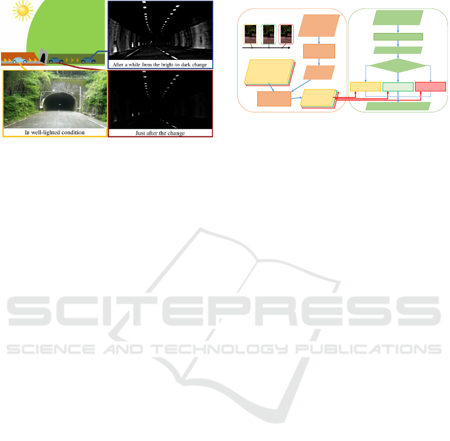
Figure 1: Simulation example of driver’s vision after bright-
to-dark illumination change.
cidents. To the best of our knowledge, this has not
been considered in previous works on the estimation
of pedestrian detectability. Figure 1 shows a simu-
lation example of a driver’s vision after the bright-
to-dark illumination change. After the change, the
driver’s visual acuity decreases during the adaptation
period until adapting to the dark illumination (Dark
adaptation). Studies on dark adaptation in the field of
psychophysics is performed by two visual functions;
“Pupillary light reflex” and “Purkinje phenomenon.”
From previous research (Rushton, 1961), it is known
that the former lasts for several seconds, while the
latter lasts for a few minutes. It implies that the
change affects the driver’s visual characteristics for
a while although he/she needs to response rapidly.
However, it might be difficult to apply the insights
from such studies to pedestrian detectability estima-
tion, since they used simple visual stimulate such as
Gabor patches and LED lights for measuring visual
sensitivity, while drivers are exposed to more com-
plex visual stimulate in real driving conditions.
The goal of our research is to estimate the pedes-
trian detectability correctly even after the illumination
changes drastically. The pedestrian detectability de-
pends on environmental variables (e.g., contrast of lu-
minance, visual adaptation period), and individual in-
ternal variables of a driver (e.g., eye sight, age). In
this paper, we focus on the visual adaptation period
since it is the most direct measure of a temporal effect
to the driver’s visual characteristics. After illumina-
tion changes drastically, a driver’s visual characteris-
tics change according to the adaptation period. So, we
proposea detectability estimation method considering
visual adaptation to drastic illumination changes. The
method constructs several estimators and estimate the
pedestrian detectability by switching them according
to the adaptation period. In summary, our contribu-
tions are as follows:
1. Introduction of driver’s visual adaptation: By
In-vehicle
camera image
Feature
extraction
Feature extraction
Pre-processing phase Estimation phase
Estimators
construction
3.0 sec.
0.5 sec.
Image
features
Image features
0.2
0.9
Pedestrian
detectability
(0.5 sec.)
1.5 sec.
0.6
Estimation
Estimation
Estimation
0.5 sec.
Adaptation period
1.5 sec.
3.0 sec.
Adaptation periods
Estimator
for 0.5 sec.
In-vehicle
camera
images
Pedestrian detectability
Pedestrian
detectability
Figure 2: Process flow of the proposed framework.
switching estimators according to the adaptation
period, the accuracy of the pedestrian detectabil-
ity estimation increases.
2. Dataset construction of the pedestrian detectabil-
ity with illumination changes: We design an ex-
perimental procedure to obtain the pedestrian de-
tectability with visual adaptation.
2 DETECTABILITY ESTIMATION
As mentioned in Section 1, after the illumination
changes drastically, the driver’s visual characteristics
change according to the adaptation period. So, the
proposed method estimates the pedestrian detectabil-
ity by switching estimators according to the adapta-
tion period. Figure 2 shows the process flow of the
proposed framework. It consists of two phases; pre-
processing phase, and estimation phase.
In the pre-processing phase, detectability estima-
tors are trained by using pairs of features and the
ground-truth of the detectability. For each adaptation
period, the ground-truthis obtained through a prelimi-
nary experiment and the estimator is trained. The esti-
mators are constructed by Support Vector Regression.
In Figure 2, the adaptation period is set to either 0.5,
1.5, or 3.0 sec.
In the estimation phase, we first measure the
driver’s gaze position and extract visual features from
an in-vehicle camera image. Then, pedestrian de-
tectability is estimated by using the estimators trained
in the pre-processing phase. To estimate consider-
ing the driver’s visual adaptation, first, drastic illu-
mination change points are detected using an illumi-
nometer. We defined the time after the change as the
driver’s visual adaptation period, and switch estima-
tors according to certain periods and estimate the de-
tectability at each period.
Feature Extraction. We apply features used in a
conventional method (Tanishige et al., 2014) for the
VISAPP 2017 - International Conference on Computer Vision Theory and Applications
612

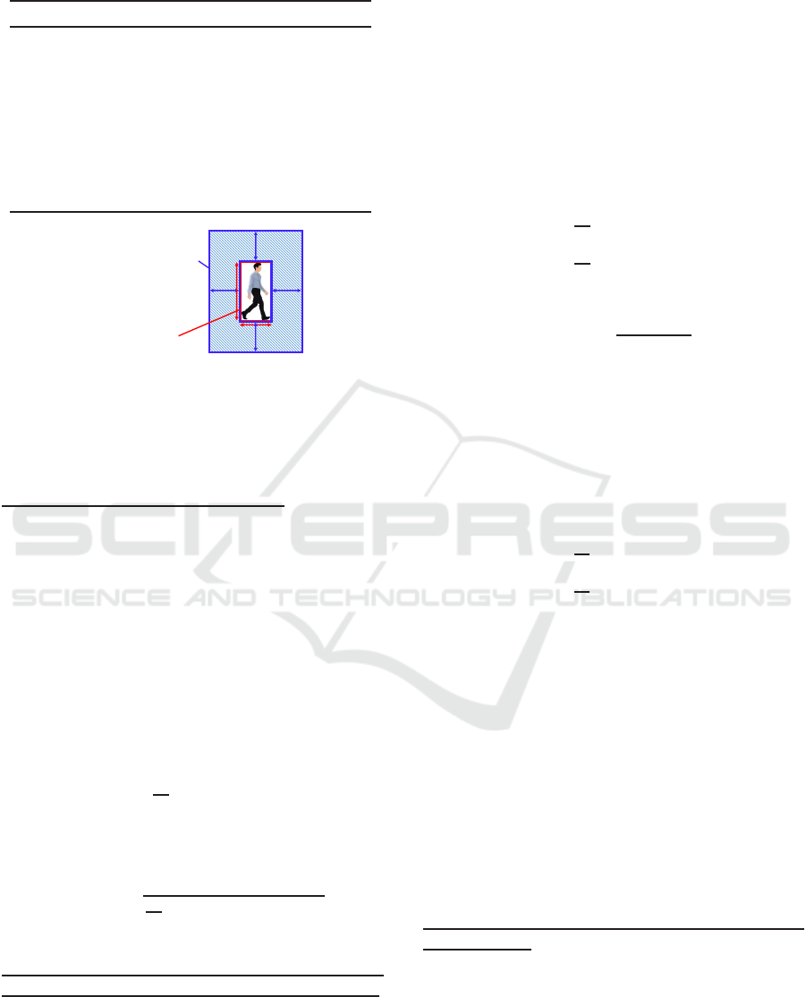
Table 1: List of features.
Abbr. Description
P
width
Width of pedestrian region
P
height
Height of pedestrian region
P
δ(lum)
Standard deviation of luminance
C
µ(lum)
Contrast of luminance
C
µ(Lab)
Contrast of average color (L*a*b*)
C
edge
Contrast of edge
C
hist(color)
Contrast of color histogram
D
(p,g)
Distance between center of the
pedestrian region and fixation point
3HGHVWULDQ¶V
surrounding region (B)
D
S
Dt
Dt
Dt
Dt
Pedestrian region (P)
Figure 3: Pedestrian region and its surrounding region.
detectability estimation. Table 1 shows the list of fea-
tures used. Here, the pedestrian region P and its sur-
rounding region B are defined as shown in Figure 3.
Features from the Pedestrian Region. In general,
the larger a pedestrian appears, and the more complex
the texture of the pedestrian region is, the easier the
driver can detect. We assume that these visual charac-
teristics influence the detectability even after a drastic
illumination change. Therefore, we extract features
related to the size of a pedestrian and its texture.
P
width
and P
height
are the width and the height of
the pedestrian region, respectively; w and h in Fig-
ure 3 .
P
σ(lum)
is the standard deviation of luminance in
the pedestrian region. First, we convert an input im-
age to an 8-bit grey scale image and calculate the av-
erage of luminance in the pedestrian region as
¯
l
P
=
1
|P|
P
(i, j)∈P
l(i, j), (1)
where |P| represents the number of pixels in region
P, and l(i, j) represents the luminance at pixel (i, j).
Then, the standard deviation P
σ(lum)
is calculated as
P
σ(lum)
=
q
1
wh
P
w
i=1
P
h
j=1
(l(i, j)−
¯
l
P
)
2
. (2)
Features of the Contrast between the Appearances
of Pedestrian Region and Its Surrounding Region.
The contrast between the appearances of a pedestrian
and its surrounding (background) is an important fea-
ture considering pedestrian detectability.
C
µ(lum)
is the contrast between the average lumi-
nance in the pedestrian region and that in the sur-
rounding region. We first calculate the average lumi-
nance in the surrounding region
¯
l
B
as with Equation
(1). Then, C
µ(lum)
is calculated as
C
µ(lum)
=



¯
l
P
−
¯
l
B



, (3)
where | · | represents the absolute value.
C
µ(Lab)
is the contrast between the average color
in the pedestrian region and that in its surrounding
region. First, we calculate the average color in the
pedestrian region ¯v
P
, and that in its surrounding re-
gion ¯v
B
, as
¯v
P
=
1
|P|
P
(i, j)∈P
v(i, j), (4)
¯v
B
=
1
|B|
P
(i, j)∈B
v(i, j), (5)
where v(i, j) is a vector in the L*a*b* color space.
Then, C
µ(Lab)
is calculated as
C
µ(Lab)
=
p
||¯v
P
− ¯v
B
||
2
, (6)
where || · || represents the Euclidean norm.
C
edge
is the contrast between the average of edge
intensity in the pedestrian region and that in its sur-
rounding region. First, Sobel filter is applied to the
grey scale image to obtain an edge intensity image.
Then, the average edge intensity is calculated in the
pedestrian region
¯
E
P
, and that in its surrounding re-
gion
¯
E
B
, as
¯
E
P
=
1
|P|
P
(i, j)∈P
E(i, j), (7)
¯
E
B
=
1
|B|
P
(i, j)∈B
E(i, j), (8)
where E(i, j) is the edge intensity at pixel (i, j). Fi-
nally, C
edge
is calculated as
C
edge
=



¯
E
P
−
¯
E
B



. (9)
C
hist(color)
is the contrast between the color his-
togram in the pedestrian region H
RGB
(P), and that in
its surrounding region H
RGB
(B), which are generated
by combining 16-bins histograms from the R, G, and
B values. Then, C
hist(color)
is calculated as
C
hist(color)
= d
EMD
(H
RGB
(P), H
RGB
(B)), (10)
where d
EMD
(H
1
, H
2
) represents the Earth Mover’s
Distance (Rubner et al., 1998).
Distance from a Pedestrian Region to the Driver’s
Gaze Position. According to psychophysics stud-
ies, the visual adaptation in the central fields-of-
view differs from that in the peripheral fields-of-view.
Therefore, we focus on the view angle from the pedes-
trian to the driver’s gaze position. The Euclidean dis-
tance between the center of the pedestrian region and
the fixation point on an input image is represented as
D
(p,g)
.
Can a Driver Assistance System Determine if a Driver is Perceiving a Pedestrian? - Consideration of the Driverâ
˘
A
´
Zs Visual Adaptation to
Illumination Change
613

Figure 4: Experimental facility (Covered with a blackout
curtain during the actual subjective experiment).
Pattern 1
Pattern 2
Pattern 3
0 1 2 3 4 5 6 7 8
(sec.)
Figure 5: Patterns of display timings of images after the
light is turned off at 0 sec. The orange horizontal bar indi-
cates the duration of displaying the image, where we obtain
the detectability.
3 DATASET CONSTRUCTION
The pedestrian detectability is the probability that a
driver perceives a pedestrian (Engel and Curio, 2012).
Since this is the measure based on human sensation,
we need to conduct a subjective experiment to obtain
the ground-truth before training the estimators. Some
works regarded the rate of detecting a pedestrian by
human subjects as the detectability (Wakayama et al.,
2012; Tanishige et al., 2014). They asked the sub-
jects to find a pedestrian in an image capturing a traf-
fic scene in stable illumination condition. Since we
focus on the visual adaptation period, we designed an
experimental environment to change the illumination
at an arbitrary timing. Figure 4 shows the facility with
controllable lights to realize the environment. During
the experiment, we covered the facility and the sub-
ject with a blackout curtain to shut out external light.
The procedure is described below.
1. The subject adapts to well-lighted environment in
the facility for 30 sec.
2. A low-resolution image capturing a traffic scene
including a non-detectable pedestrian is displayed
to the subject.
3. The subject is instructed to fix his/her eye gaze at
a certain position indicated by a cross.
4. The illumination is drastically changed by turning
off the lights.
5. After T [sec.], a high-resolution image of the
same scene as Step 2. is displayed for 0.5 sec.
6. The subject searches the pedestrian in the image.
Figure 6: Examples of images in the dataset.
7. The subject indicates the position of the pedes-
trian by touching the display.
8. The cross is displayed again, then Steps 2. to 7.
except for Step 4., are repeated once more with
another image.
We displayed the low-resolution image of the
same scene as the high-resolution image to reduce the
effect of visual surprise. We conducted the procedure
with T = 0.0, 1.0, 2.5, 4.0, 5.5, and 7.0 sec. For ef-
ficiency of time, we displayed two scenes (the first
one with, and the second one without illumination
change) in a single procedure. Hence, we obtained
the detectability corresponding to six adaptation peri-
ods by carrying out the procedure with three patterns
of display timings of images as shown in Figure 5. In
addition, we fixed the luminance in the well-lit envi-
ronment to about 1,000 luxes, that is, the luminance
at an hour before sunset, and that in the dark environ-
ment with about 10 luxes to reproduce twilight gloom.
We used a camera (iVIS HF G10, Canon Inc.)
to capture traffic scenes in twilight. Then we manu-
ally extracted frames containing one pedestrian from
the videos. Figure 6 shows four examples of images
whose resolution is 1,920 × 1,080 pixels. We also
used an organic electroluminescent display (arrows
Tab F-03G, Fujitsu Inc., 10.5 inches, 2,560 × 1,600
pixels, 2,000,000:1 contrast ratio) with touch panel to
display the images, and some lights (Grassy LeDiO
RX122 FleshWhite, Volxjapan Co. Ltd. and Hue,
Philips) to control the illumination condition.
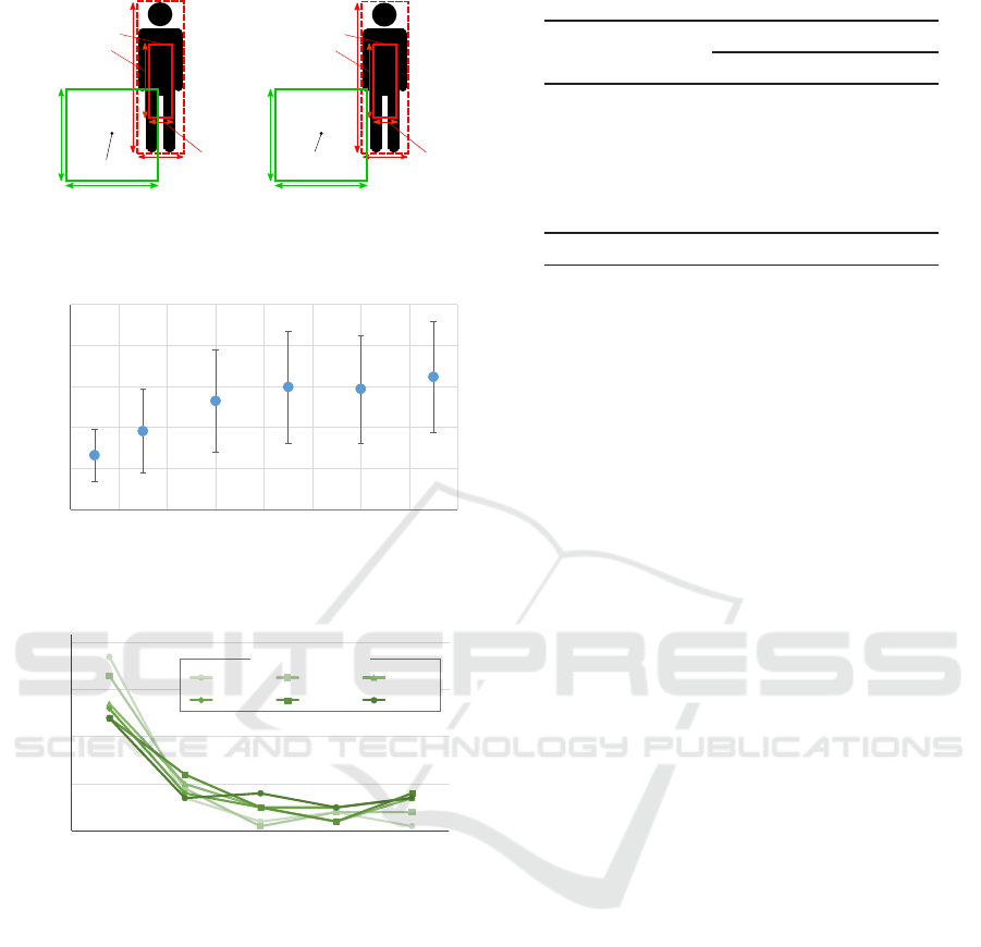
Figure 7 shows a criterion to judge whether the
subject’s response is correct or not. We defined a
center region of the pedestrian region as ground-truth,
and a 200 pixels
1
square around the touched point as
the response region. If it overlapped with the ground-
truth, it was regarded as correct. Then we calculated
the rate of correct responses by all subjects as the
pedestrian detectability.
We conducted this experiment with four subjects
(three males and one female) with normal vision
1
Corresponds to about five degs. in the visual field.
VISAPP 2017 - International Conference on Computer Vision Theory and Applications
614

h
w
h/2
w/2
200
200
Pedestrian region
Ground-truth region
Input point
Response region
(a) Example of correct.
h
w
h/2
w/2
200
200
Pedestrian region
Ground-truth region
Input point
Response region
(b) Example of incorrect.
Figure 7: Criterion for the judgement of the subject’s re-
sponse.
0.0
0.1
0.2
0.3
0.4
0.5
0 1 2 3 4 5 6 7 8
Pedestrian detectability
Adaptation period (sec.)
Figure 8: Relation between the pedestrian detectability and
the adaptation period.
0
10
20
30
40
0.00 0.25 0.50 0.75 1.00
Number of pedestrians
Pedestrian detectability
0.5 sec. 1.5 sec. 3.0 sec.
4.5 sec. 6.0 sec. 7.5 sec.
Adaptation periods
Figure 9: Distribution of the pedestrian detectability for
each adaptation period.
whose ages ranged between 22 and 30. In this ex-
periment, we prepared 51 images containing just one
pedestrian in each of them. Thus we obtained 306
ground-truth data, i.e., 51 pedestrians for each of six
adaptation periods, of the pedestrian detectability.
Figure 8 shows the relation between the obtained
pedestrian detectability and the adaptation period.
Here, the points and lines represent the average and
variance of the pedestrian detectability of 51 pedes-
trians, respectively. From this result, we can say that
the pedestrian detectability increased gradually until
4.5 sec. in this experiment. As mentioned in Sec-
tion 1, the dark adaptation is performed by the fol-
lowing two visual functions; “Pupillary light reflex”
and “Purkinje phenomenon.”The former lasts for sev-
eral seconds, while the latter lasts for a few minutes
Table 2: Evaluation result.
Adaptation period
Mean Squared Error
Proposed Comparative
0.5 sec. 0.069 0.066
1.5 sec. 0.108 0.110
3.0 sec. 0.134 0.144
4.5 sec. 0.144 0.177
6.0 sec. 0.140 0.169
7.5 sec. 0.141 0.185
Avg. 0.123 0.134
(Rushton, 1961). We therefore infer that this result
reflected the visual recovery of the former.
Figure 9 shows the distributions of the pedestrian
detectability for each adaptation period. This result
indicates that the longer the adaptation period is, the
less the number of pedestrians which has zero de-
tectability is.
4 RESULT AND DISCUSSION
To construct the multiple estimators for the proposed
method, we divided the dataset into six groups ac-
cording to the adaptation periods and trained six es-
timators using each group. To evaluate the proposed
method considering the visual adaptation, we com-
pared the estimation error with a comparative method
which used a single estimator trained with all of
the detectability data, in a similar way to previous
studies (Engel and Curio, 2012; Wakayama et al.,
2012). Leave-one-pedestrian-outcross validation was
applied that is 50 pedestrians were used for training
and one pedestrian for testing.
Table 2 shows the comparison of the estimation
error for each adaptation period between the proposed
method and the comparative method. The estimation
errors in which the adaptation period was 0.5 and 1.5
sec. were low for both methods. On the other hand,
focusing on the longer 3.0 sec., the proposed method
had lower error than the comparative method. The
estimators might have overfit to the dataset because
it had a large bias in the detectability distribution for
which the adaptation period was 0.5 and 1.5 sec.
For discussion, we analyzed the effectiveness of
the features for each adaptation period. In detail, we
first chose a couple of features from the eight visual
features, then constructed estimators correspondingto
the adaptation period and evaluated them. This pro-
cedure was applied to all combinations of features
(
8
C
2
= 28). Finally we placed them in ascending or-
der of the estimation error.
Table 3 shows the order and Mean Squared Er-
Can a Driver Assistance System Determine if a Driver is Perceiving a Pedestrian? - Consideration of the Driverâ
˘
A
´
Zs Visual Adaptation to
Illumination Change
615

Table 3: Order of the pair of image features (Evaluated by Mean Squared Error).
Order
Adaptation period
0.5 sec. 1.5 sec. 3.0 sec. 4.5 sec. 6.0 sec. 7.5 sec.
1
P
δ(lum)
,C
edge
C
µ(Lab)
,C
edge
P
δ(lum)
,C
µ(lum)
P
δ(lum)
,C
µ(lum)
P
δ(lum)
,C
µ(lum)
P
δ(lum)
,C
µ(lum)
0.047 0.060 0.063 0.084 0.081 0.059
2
P
δ(lum)
,C
µ(lum)
P
δ(lum)
,C
edge
P
δ(lum)
,C
µ(Lab)
P
height
,C
µ(Lab)
P
δ(lum)
,C
µ(Lab)
P
δ(lum)
,C
µ(Lab)
0.052 0.061 0.067 0.103 0.087 0.083
3
P
width
,C
edge
P
δ(lum)
,C
µ(Lab)
P
width
,C
edge
P
δ(lum)
,C
µ(Lab)
P
height
,C
µ(Lab)
P
width
,C
edge
0.059 0.069 0.071 0.106 0.107 0.104
ror of each combination. This result indicates that af-
ter 3.0 sec., C
µ(lum)
and C
µ(Lab)
contributed to achieve
lower estimation error. On the other hand, just after
0.5 and 1.5 sec., C
edge
contributed. This also indi-
cates that the same combinations achieved low error
after 3.0 sec. Hence it is inferred that after 3.0 sec.,
the change of visual characteristic would be small.
5 CONCLUSION
In this paper, we proposed a method for the estimation
of pedestrian detectability considering visual adapta-
tion to drastic illumination changes, and indicated that
a driver assistance system can determine if a driver is
perceiving a pedestrian to some extent. Specifically,
the proposed method extracts visual features and es-
timates the pedestrian detectability by switching the
estimators according to the adaptation period.
To evaluate the proposed method, we first con-
structed an experimental environment to present a
subject with drastic illumination changes and then
conducted an experiment to measure and estimate the
pedestrian detectability according to different adap-
tation periods. Evaluation results showed that the
proposed method considering the visual adaptation
was effective for the estimation of the pedestrian de-
tectability. In addition, we analyzed the effective fea-
tures for each adaptation period.
In future work, we will introduce additional fea-
tures based on physiological knowledge, and conduct
subjectiveexperiments to expand the dataset. Further-
more, we will apply the obtained knowledge to an ac-
tual vechicle to validate the application possibility.
ACKNOWLEDGEMENTS
Parts of this research were supported by JSPS Grant-
in-Aid for Scientific Research, MEXT.
REFERENCES
Arumi, P., Chauhan, K., and Charmant, W. (1997). Ac-
commodation and acuity under night-driving illumi-
nation levels. Ophthalmic and Physiological Optics,
17(4):291–299.
Engel, D. and Curio, C. (2012). Detectability prediction in
dynamic scenes for enhanced environment perception.
In Proc. 2012 IEEE Intelligent Vehicles Symposium,
pages 178–183.
NHTSA’s National Center for Statistics and Analysis
(2015). Critical reasons for crashes investigated in the
national motor vehicle crash causation survey.
Rohling, H., Heuel, S., and Ritter, H. (2010). Pedestrian
detection procedure integrated into an 24 ghz automo-
tive radar. In Proc. 2010 IEEE Radar Conf., pages
1229–1232.
Rubner, Y., Tomasi, C., and Guibas, L. J. (1998). A metric
for distributions with applications to image databases.
In Proc. 6th Int. Conf. on Computer Vision, pages 59–
66.
Rushton, W. A. H. (1961). Rhodopsin measurement and
dark-adaptation in a subject deficient in cone vision.
J. Physiology, 156(1):193–205.
Tanishige, R., Deguchi, D., Doman, K., Mekada, Y., Ide, I.,
and Murase, H. (2014). Prediction of driver’s pedes-
trian detectability by image processing adaptive to vi-
sual fields of view. In Proc. 17th IEEE Int. Conf. on
Intelligent Transportation Systems, pages 1388–1393.
Viola, P., Jones, M. J., and Snow, D. (2005). Detecting
pedestrians using patterns of motion and appearance.
Int. J. of Computer Vision, 63(2):153–161.
Wakayama, M., Deguchi, D., Doman, K., Ide, I., Murase,
H., and Tamatsu, Y. (2012). Estimation of the human
performance for pedestrian detectability based on vi-
sual search and motion features. In Proc. 21st IAPR
Int. Conf. on Pattern Recognition, pages 1940–1943.
Wegner, A. J. and Fahle, M. (1999). Alcohol and visual per-
formance. Progress in Neuro-Psychopharmacology
and Biological Psychiatry, 23(3):465–482.
World Health Organization (2015). Global status report on
road safety 2015.
VISAPP 2017 - International Conference on Computer Vision Theory and Applications
616