Empirical Evaluation of Convolutional Neural Networks Prediction Time

in Classifying German Trafﬁc Signs

Joshua Fulco

, Akanksha Devkar

, Aravind Krishnan

, Gregory Slavin

and Carlos Morato

1,3

Robotics Engineering Department, Worcester Polytechnic Institute, Worcester, MA 01609, U.S.A.

Electrical and Computer Engineering Department, Worcester Polytechnic Institute, Worcester, MA 01609, U.S.A.

Department of Mechatronics and Sensors, US Corporate Research Center, ABB Inc., CT 06002, U.S.A.

Keywords:

Convolutional Neural Networks, Classiﬁcation Time, Trafﬁc Sign Classiﬁcation.

Abstract:

This paper discusses the use of Deep Learning and neural networks to identify images which contain road signs

to aid in the navigation of autonomous vehicles. Images of 32x32 pixels and 128x128 pixels of the GTSRB

dataset were used in training the existing neural network models as well as our novel models. Existing neural

network models mentioned in the literature study validate that very high accuracies in image classiﬁcation

are already achieved. Different neural network model architectures were also reviewed to determine which

architecture produced the highest accuracy within the most efﬁcient time. Modiﬁcations to these architectures

were made to produce valid results with a reduced image identiﬁcation time. Our results of classifying a trafﬁc

sign image of 32x32 pixels in 0.6ms is very reliable for real time output. By looking at the image identiﬁcation

times for a 32x32 pixel image and a 128x128 pixel image we observed that size of the image is not the main

factor in the increase of the prediction time.

1 INTRODUCTION

Deep learning is a form of machine learning which

has recently re-emerged as a topic of great interest

and advanced research around the world after a near

decade fallout with researchers. The basic concept of

machine learning also known as representative learn-

ing can be best described in an example where a ma-

chine (or system of machine processors) takes in raw

data such as an audio clip or photograph and then

uses extractor tools to discover patterns within the raw

data. Features identiﬁed or discovered within the raw

data by the machine are passed between the multi-

ple layers or ﬁlters which are used to sort out features

such that they are saved to memory. In theory, with

a varying degree of accuracy, a system exercising the

methods of machine learning should be able to recog-

nize and/or identify identical or similar data to what

was presented in a previous training. In many ways

machine systems which are organized in a manner

similar to how it is believed the human brain is or-

ganized to intake information. It is believed that the

neurons in the human brain accept data or information

through the dendrites. The nucleus sorts or identi-

ﬁes this information and then transmits other portions

of the information through impulses sent out to other

neurons through axons. With machine learning ﬁlters

or activation functions which identify features in raw

data are often organized in layers. These ﬁlters usu-

ally are trained to identify one particular feature, and

pass other information between activation functions

in the layer or transmit binary signals conﬁrming or

eliminating the presence of a feature on to the next

layer or back to a previous layer. Methods with at

least three layers of activation function ﬁlters are re-

ferred to Deep learning models.

Deep learning methods are making great strides

recently in the ﬁeld of autonomous automotive op-

erations. Recent news has been made with record

breaking deliveries for the Anheuser-Busch Corpora-

tion using autonomous vehicles (Menge, 2016). Deep

learning methods of machine learning have also been

used to aid in navigation of sedan vehicles on roads

with varying terrain. As shown in source (Bojarski

et al., 2017) a series continuously taken photographs

of a vehicles path are used to determined wheel orien-

tation. The photograph data is used to train a naviga-

tion model which can correlate to wheel position. In

addition visual navigation from images along a path

are hoped to mature as autonomous vehicle devel-

opment continues. Street sign recognition through

Deep Learning can also be used for vehicle veloc-

ity and navigation control, such that an autonomous

vehicle will stop at a stop sign, yield to a pedestrian

260

Fulco, J., Devkar, A., Krishnan, A., Slavin, G. and Morato, C.

Empirical Evaluation of Convolutional Neural Networks Prediction Time in Classifying German Trafﬁc Signs.

DOI: 10.5220/0006307402600267

In Proceedings of the 3rd International Conference on Vehicle Technology and Intelligent Transport Systems (VEHITS 2017), pages 260-267

ISBN: 978-989-758-242-4

or other vehicles, as well as identify directional route

signs and road placards on a highway. It is the subject

of this paper to exploit the development of a Convo-

lutional Neural Network Deep Learning model that

could possibly be used to identify road signs for use

in the navigation of autonomous vehicles.

2 OBJECTIVE

It’s about time that we have autonomous cars taking

on the roads and the technology today has certainly

evolved to the extent of realising robotic cars unleash

the Earth’s road networks. Lux Research calculates

that the revenue opportunity from Advanced Driver

Assistance Systems (ADAS) features will grow from

$2.4 billion today to $102 billion in 2030. For such

an autonomous car to perform efﬁciently, it needs to

perceive the road visually. These cars need to have a

sharp vision that detect all types of road conditions -

trafﬁc lights, road signs and take corrective measures

accordingly. Also, we have recently seen that Tesla’s

semi-autonomous cars are performing great with their

Autopilot mode and this assistance relieves drivers

stress.

Semi-autonomous cars are excelling in keeping

the driver alert by suggesting corrective actions and

making sure the driver doesn’t miss any on-road in-

formation. We focus on reducing the space and time

complexity of classiﬁcation of German road signs us-

ing one of the Deep Learning techniques - Convo-

lutional Neural Networks(CNN) for the purpose of

driver assistance and making an autonomous car more

efﬁcient.

Staggering results are achieved in the ofﬂine clas-

siﬁcation reaching 99.65% (Mao et al., 2016) accu-

racy, and when these results are compared with the

real-time classiﬁcation results, they are low, partic-

ularly due to the computational complexity in time

and hardware requirements. It is varying anywhere

between 80% to 93% (Chen et al., 2012). After lo-

calization and detection, the detected image of a road

sign can have problems like

Scaling - leads to image quality reduction making

it hard to recognize/discern.

Rotation - a damaged/ rotated sign may be inter-

preted as a different sign altogether, for instance when

a left arrow somehow rotated 90 degrees clockwise

can simply mean that it is a straight arrow and not

make any sense. It is much harder to understand if

that rotated arrow was pointing right or left originally.

Projection distortion - a distorted sign board can

lead to wrong classiﬁcation or no classiﬁcation, for

instance the sign which indicates the merging of

left/right lane can be classiﬁed completely wrong due

to the distortion in the top portion of the sign.

There are few other problems while detecting the

road signs during the video recording phase such as

road signs may be subjected to dust deposition, or

may have faded with time, or be victim to grafﬁti,

stickers subjecting to occlusion and even getting dam-

aged in some cases. All these lead to increase in

the error rates of detection, prediction and classiﬁ-

cation process. So we believe, Deep Learning with

CNN on a good hardware with reduced algorithmic

complexity can ease the process and improve accu-

racy for the real-time output. Another aspect to con-

sider is the selection of a dataset or datasets. Most

of the Deep Learning road sign identiﬁcation exper-

iments we found are based on a German set of road

signs known as the German Trafﬁc Sign Recogni-

tion Benchmark (GTSRB) (Igel, ) which has become

somewhat of a standard bearer.

As mentioned above, real time road sign detec-

tion is an important feature on ADAS, but in order

to be truly effective it needs to be both, accurate

and efﬁcient. Speciﬁcally for road sign classiﬁcation,

Deep Learning models based on Neural Networks are

known to be very accurate, achieving rates above hu-

man detection abilities (according to our preliminary

research) but not necessarily fast enough (yet) to be

used in real time systems where (embedded) process-

ing power is limited. On the other side, more con-

ventional computer vision techniques can be used to

achieve real time processing speed, but fell short in

accuracy when compared to Deep Learning methods.

Our objective is to empirically evaluate different Con-

volutional Neural Networks with multiple variations

of the hyper-parameters and make it classify the road

signs more efﬁciently for the real time output.

3 REVIEW OF LITERATURE

Dan Cires et al. avoided the cumbersome computa-

tion of handcrafted features and achieved a 98.73%

recognition rate with the best of their CNNs for the

German road sign recognition benchmark. They fur-

ther improved these results up to 99.15% recognition

rate using a committee of a CNN and a Multi Layer

Perceptron(MLP) where the CNNs are trained on raw

pixel intensities, although error rates of the best MLPs

are 3-4% above those of the best CNNs, a commit-

tee consistently outperforms the individual classiﬁers.

(Ciresan et al., 2011)

Jack Greenhalgh et al. proposed a novel real-time

system for the automatic detection and recognition

of trafﬁc symbols. Candidate regions are detected as

Empirical Evaluation of Convolutional Neural Networks Prediction Time in Classifying German Trafﬁc Signs

261

MSERs. This detection method is signiﬁcantly insen-

sitive to variations in illumination and lighting con-

ditions. Trafﬁc symbols are recognized using HOG

features and a cascade of linear SVM classiﬁers. A

method for the synthetic generation of training data

was proposed, which allows large datasets to be gen-

erated from template images, removing the need for

hand labeled datasets. Their system can identify signs

from the whole range of ideographic road signs cur-

rently in use in the U.K. which form the basis of our

training data. This system retains a high accuracy at

a variety of vehicle speeds and achieved recognition

accuracy of 89.2% for white road signs and 92.1% for

color signs (Greenhalgh, 2012)

Tam T. Le et al. presented a real-time process-

ing method of trafﬁc-sign detection to apply in au-

tonomous driving system. Their proposed method uti-

lized linear SVM to classify color by a low complex-

ity (average 23 ms per frame). After that shape match-

ing was applied to eliminate positive errors. They

achieved 92.91 percent of detection accuracy and it

was applied on real-time autonomous driving system

with the processing speed of 20fps, where the maxi-

mum speed of car was limited at 30 km per hour.(Le

et al., 2010)

Yujun Zeng et al. proposed a novel architecture

for road sign recognition, where CNN acts as a fea-

ture extractor and Extreme Learning Machines(ELM)

trained on CNN-learnt features as the classiﬁer, so

that the discriminative Deep Convolutional features

could match well with the generalization performance

of ELM classiﬁer, leading to a satisfactory recogni-

tion accuracy without using more complex CNNs, en-

semble features, or data augmentation. In contrast

with state-of-art methods, the proposed method could

achieve competitive results (99.40%, without any data

augmentation and preprocessing like contrast normal-

ization) with a much simpler architecture that relieves

the time-consuming training procedure a lot. Yet, the

fact that most errors are mainly due to motion blur im-

plies that the performance may be further improved

if the CNN is equipped with some layers that could

learn blur-invariant features.(Zeng et al., 2015)

Pierre Sermanet et al. presented a Convolu-

tional Network architecture with state-of-art results

on the GTSRB road sign dataset implemented with

the EBLearn open-source library. During phase I

of the GTSRB competition, this architecture reached

98.97% accuracy using 32x32 colored data while

the top score was obtained by the IDSIA team with

98.98%. The ﬁrst 13 top scores were obtained with

ConvNet architectures, 5 of which were above human

performance (98.81%).

Subsequently to this ﬁrst phase, they established

a new record of 99.17% accuracy by increasing net-

works capacity and depth and ignoring color informa-

tion. This contradicted prior results with other meth-

ods suggesting that colorless recognition, while ef-

fective, was less accurate. They also demonstrated

the beneﬁts of multi-scale features in multiple exper-

iments. Additionally, they report very competitive

results (97.33%) using random features.(Sermanet,

2011)

Junqi Jin et.al designed a TSR system using a

CNN, which is a special kind of deep neural net-

work. The model had the ability to learn both fea-

tures and classiﬁers. The learned features detect spe-

ciﬁc local patterns that are better than hand-coded fea-

tures. They have proposed an Hinge Loss Stochastic

Gradient Descent (HLSGD) method to train CNNs.

After they tested their algorithm on the GTSRB and

compared results with other competitors, their exper-

iments showed that HLSGD gave faster and more sta-

ble convergence and a state-of-art recognition rate of

99.65%(Jin et al., 2014)

4 DATASET

With any Deep Learning model a compiled set of raw

data is necessary to train, test, and validate a model.

The more samples within a dataset, the more features

a model can recognize during training. (Provided the

samples belong to a small number of classes.) The

more features recognized by the model, the better the

chance of high accuracy sample recognition during

validation and actual use. Due to access and time the

availability of compiled datasets is limited. It is not

uncommon for researchers to modify existing datasets

to achieve a large number of samples. In the case of

an image dataset it is not uncommon for images to be

cropped, contracted to a smaller size or speciﬁc area,

or reduced to gray scale if in color.

Traditionally half of a dataset is used for the pur-

poses of training. The remaining half is again split

into quarters. One quarter is used as part of a test set,

which may be mixed with the training set to determine

system accuracy following training. If the model does

not recognize the test set with the accuracy desired

additional exposure to the training set may occur un-

til the desired accuracy is achieved. The last quarter

of a dataset, is often referred to as the validation set.

This set of data is not used until training is complete.

The validation set is exposed to the model for identi-

ﬁcation to serve as a ﬁnal proof of model accuracy.

For this project, to train a Deep Learning model

that can identify road signs, an image dataset was re-

quired. Two image datasets were found to be in exis-

VEHITS 2017 - 3rd International Conference on Vehicle Technology and Intelligent Transport Systems

262

tences that are used by commercial groups in pursuit

of autonomous vehicle navigation. The ﬁrst dataset

is from the Laboratory for Intelligent and Safe Auto-

mobiles (LISA) at the University of San Diego Cal-

ifornia, a group funded by a grant from several auto

manufacturers and US government agencies. Dataset

(Trivedi, ) is derived from several videos which were

recorded from car dashboard cameras. Some sample

datasets were parsed into individual still images. As

a result 47 types of US road signs are recorded in im-

ages with the natural scenic background. The images

range in size from 640x480 to 1024x522 pixels. 6610

images are in the set with 7855 annotations that iden-

tify the content of the images. Annotation content in-

cludes not only road sign descriptions but descriptions

of other items seen in the frame.

The second dataset is the German Trafﬁc Sign

Recognition Benchmark (GTSRB) dataset, contain-

ing 40 classes of German trafﬁc signs, and 50,000

images ranging in size from 15x15 to 250x250 pix-

els.(Stallkamp et al., 2012) The dataset was ﬁrst used

as a benchmark for the 2011 IJCNN computer vision

competition, and is provided by the real time com-

puter vision research group. The dataset has both sin-

gle and multi-annotated images of road signs only.

The road signs are photographed in natural environ-

ments, but cropped so show only the signs. Natural

environments do include various lighting and weather

conditions.

We decided to train the model used for this ex-

periment with the LISA dataset but after realizing

that the dataset was very small relative to other im-

age datasets that were used for successful identiﬁca-

tion with Deep Learning, a plan to combine the GT-

SRB with the LISA dataset was compiled. During

the early phases of the effort it was realized that the

two datasets only have one class of sample image in

common. Stop signs are the same in both the United

States as well as in Germany. Simply increasing the

number of classes with a small number of images in

a dataset (as would result from a simple combination

of both datasets) will not yield more accurate results

at training, as not enough features will be discovered

to improve identiﬁcation accuracy.

It was also realized that the datasets contain image

samples that were different in focus and size. The GT-

SRB samples have only a ten percent border around

the sign, while the LISA samples and more gener-

ically pictures with road signs in the image frame.

As such to combine the datasets the stop signs in the

LISA dataset would need to be reduced and cropped

to have a matching size to the other dataset. It was de-

termined that the effort of combining the two datasets

was not an efﬁcient use of time as the images gained

in the new dataset would be less than three percent of

the images already contained in the GTSRB dataset.

As such only the GTSRB dataset was used for im-

age identiﬁcation in the project. All references to the

dataset will reference the GTSRB. While the break-

down of the dataset for training, test, and validation

as noted above is the accepted standard, processor ca-

pability limited the ability to work with whole sets.

Sample images from the dataset were loaded to work

with the model in batches containing 4000 to 6400

samples accordingly.

5 IMPLEMENTATION DETAILS

Three main Python scripts were used to produce the

bulk of the work. The ﬁrst script was used to build a

workable version of the dataset to be used for train-

ing, based on the original GTSRB dataset. The path

and names of all the images with their corresponding

class were collected from the annotation ﬁle provided.

The localization and dimensions of the trafﬁc signs in

each image were again obtained from the annotation

ﬁles. For convenience, 43 separate folders were cre-

ated and the respective trafﬁc sign (also called classes)

images were resized to predetermined size of 32x32

and 128x128 pixels and stored respectively.

The second script was used to train the GTSRB

dataset using a combination of Convolutional Neural

Network models and image sizes. An augmented ver-

sion of this GTSRB dataset was developed by rota-

tion of the images in various angels. In preparation

for the training, a list of all the image ﬁlenames were

created and shufﬂed for randomness. This increased

the robustness of the network. The process of training

was performed in batches where the image ﬁles were

loaded into memory, divided as training, validation

and testing sets with a factor of , and respectively.

At the very end, the model with its weights were saved

to a .h5 ﬁle. For plotting purposes, the history and the

scores’ results were saved to .npy ﬁles.

The third script performs the actual class predic-

tion time measurements. Just like the training script

(second script), the process starts by creating the ran-

dom list of image ﬁles and loading the test set to be

used for prediction. The ﬁle saved by the training

script is used to load the desired model and then each

sample, or a collection of samples from the test set are

then submitted for prediction having their execution

time collected using the timeit Python library. Time

results are saved in a .npy ﬁle to be processed later.

This process is then repeated for each trained model

selected and we had six different models.

Empirical Evaluation of Convolutional Neural Networks Prediction Time in Classifying German Trafﬁc Signs

263

6 MODEL TRAINING

(INTERMEDIATE RESULTS)

As part of our study of prediction times for real-time

applications, for instance in detection and classiﬁca-

tion of trafﬁc signs for an autonomous vehicle, we

used a variety of convolutional neural network models

with distinct characteristics. We were speciﬁcally in-

terested in gathering information about the prediction

time itself.

Six models were used, with the total number of

layers ranging from 3 to 31, more speciﬁcally from

1 to 10 convolutional layers. The training used two

versions of the dataset with images previously resized

to 32x32 pixels and 128x128 pixels. The dataset was

divided into 50% for the training, 25% for the vali-

dation and 25% for the testing. All the six models

were trained on a Intel i7 processor with NVIDIA

GPU 1060 series. the physical RAM was about 16

gigabytes. All the models converged for the normal

dataset(without augmentation). Typically the deeper

models took more than 24 hours to complete the train-

ing. The shallowest model 1 took about 6 hours to

ﬁnish training. The ﬁnal, trained, models had a num-

ber of parameters varying from a little more than 300

thousand up to almost 70 million. A brief summary of

the models used is listed in Table 1, where the number

of convolutional layers is the most important aspect.

Table 1: Convolutional Network Models.

Model Layers Parameters

Total Convolutional 32 Pixels 128 Pixels

1 3 1 1,239,339 28,846,315

2 10 2 319,979 7,397,867

3 31 10 28,463,723 59,921,003

4 16 4 1,482,091 17,210,731

5 16 4 5,835,435 68,749,995

6 17 3 3,788,907 54,120,555

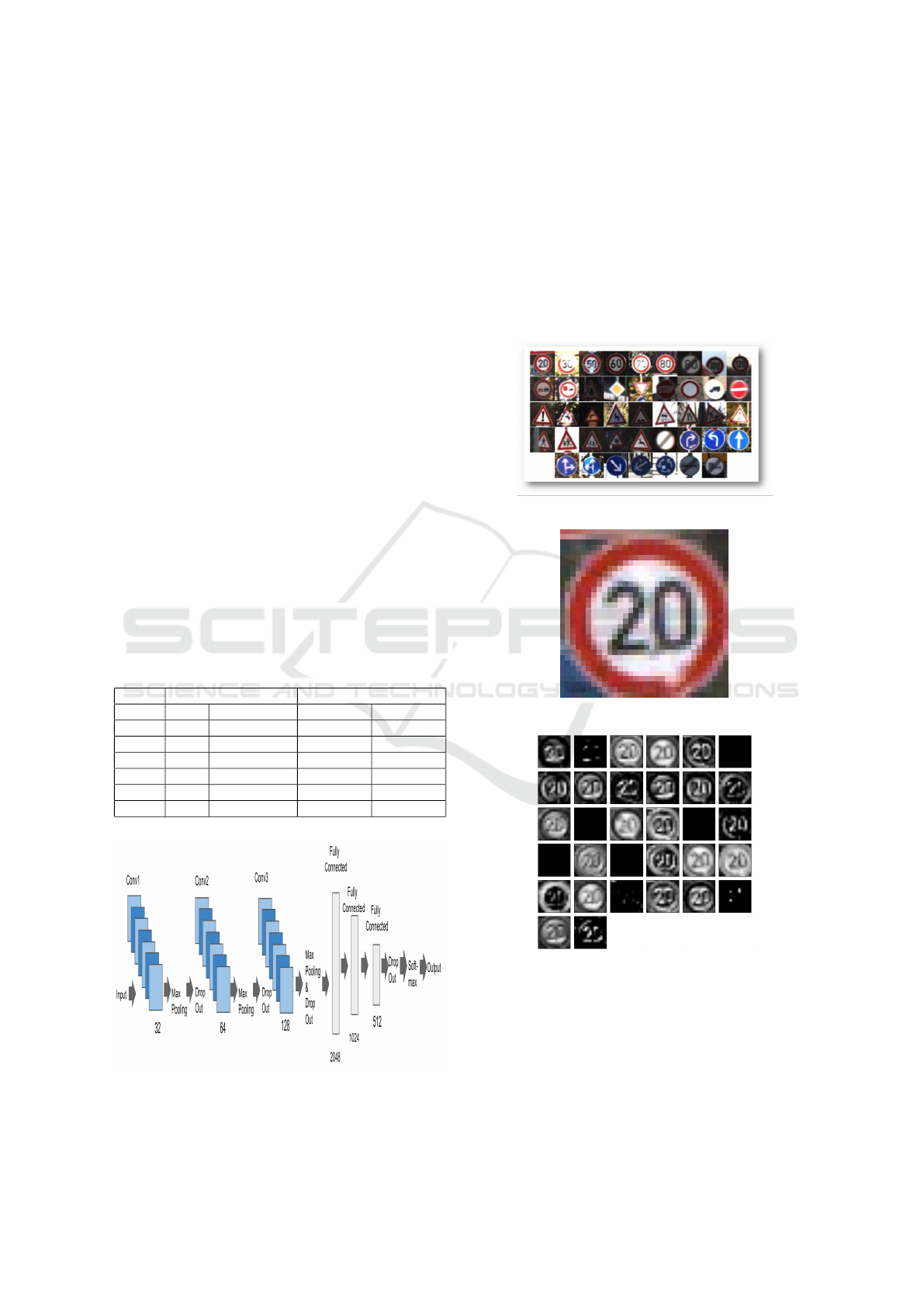
Figure 1: Model 6 Architecture.

Fig. 1 shows the architecture of our best model-

the model 6 and Fig. 2 shows the instances from GT-

SRB dataset. We considered one of the trafﬁc signs,

’Speed Limit of 20kmph’ as shown in Fig. 3 and ob-

tained visualizations per layer for model 6. Fig. 4

shows the ﬁrst layer i.e. the Convolutional Layer with

32 ﬁlters. Convolutional layer computes the output

of neurons that are connected to local regions in the

input, each computing a dot product between their

weights and a small region they are connected to in

the input volume.

Figure 2: Instances from GTSRB dataset.

Figure 3: Trafﬁc Sign - Speed Limit of 20kmph.

Figure 4: First Layer: Convolutional Layer with 32 ﬁlters.

Fig. 5 shows the second layer i.e. Max Pooling

layer that performs a downsampling operation along

the spatial dimensions (width, height), and ﬁg. 6

shows the eighth layer that applies Max Pooling after

the third and ﬁnal convolutional layer with 128 ﬁlters

Fig. 7 shows validation accuracy results for a combi-

nation of models and image sizes, where a rate of 99%

VEHITS 2017 - 3rd International Conference on Vehicle Technology and Intelligent Transport Systems

264

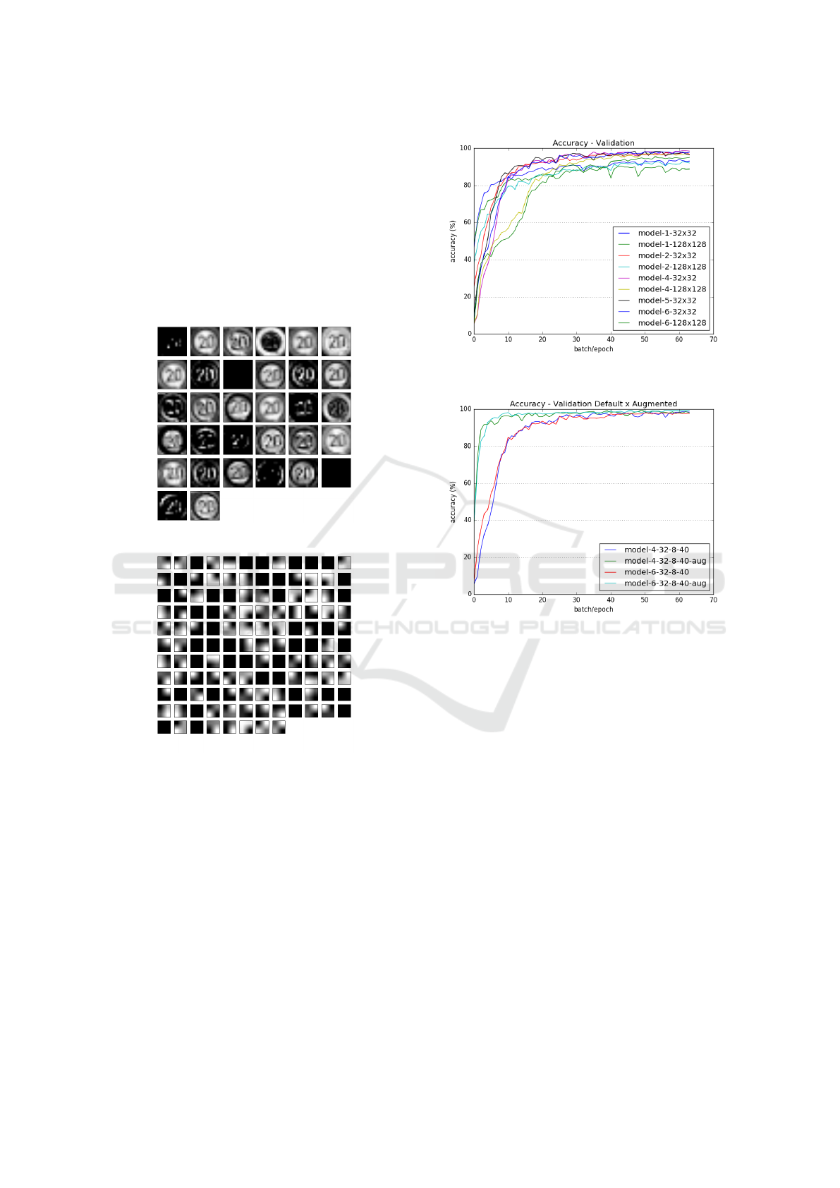
was achieved in a few cases. Training with a higher

number of epochs also showed a slight improvement

in overall accuracy. Additionally, an augmented ver-

sion of the dataset, by means of small rotation on the

original images, was also used for training, hoping for

better accuracy. In the experiment, image rotations

of -4o,-2o,+2o and +4o were added to the dataset at

training time. Two of the best models in respect to ac-

curacy, were then selected for training this augmented

version of the dataset. Improved accuracy results are

shown in Fig. 8.

Figure 5: Second Layer: Max Pooling.

Figure 6: Eighth Layer: Max Pooling.

7 RESULTS - PREDICTION AND

MEASUREMENT

After having trained multiple models, in different sce-

narios, we started performing class prediction time

measurements. Using the trained models and a subset

of the test set, the prediction time was measured, at

ﬁrst, sample by sample.

The results from all 6 models are shown in Fig.

9. The left side of the image shows the prediction

times for samples with 32x32 pixels and samples with

128x128 pixels on the right. Prediction times varied

from as low as 0.6ms for the ﬁrst model up to about

Figure 7: Accuracy for Validation Set.

Figure 8: Augmented x Non-Augmented Accuracy.

11.5ms for the 3rd model in the case of images with

32x32 pixels. If we consider a scenario where each

video frame has an average of 3 trafﬁc signs, they

are equivalent to processing 500fps down to 30fps. In

the case of 128x128 pixel images, when compared to

the 32x32 pixel images, prediction times increased to

2.3ms for the ﬁrst model and up to 21.0ms for the 3rd

model, or in video processing terms, 140fps down to

15fps. The increase in time was about 1.3 times for

the best case, up to 7.5 times for the worst case. The

model 3 happens to be the shallowest of the 6 mod-

els. One important observation made here is, in most

cases the prediction time increase was less than 2.5

times when compared to the increase in image size of

16 times in the number of pixels. It shows that the

image size is not the main factor behind the increase

in prediction times.

Up to this point, all time measurements (and train-

ing) were performed on a system based on a NVIDIA

GTX 1060 GPU card with 6GB of memory. To

better understand the variations in hardware perfor-

mance, additional experiments were performed with

other GPU and CPU based systems. Fig. 10 shows

Empirical Evaluation of Convolutional Neural Networks Prediction Time in Classifying German Trafﬁc Signs

265

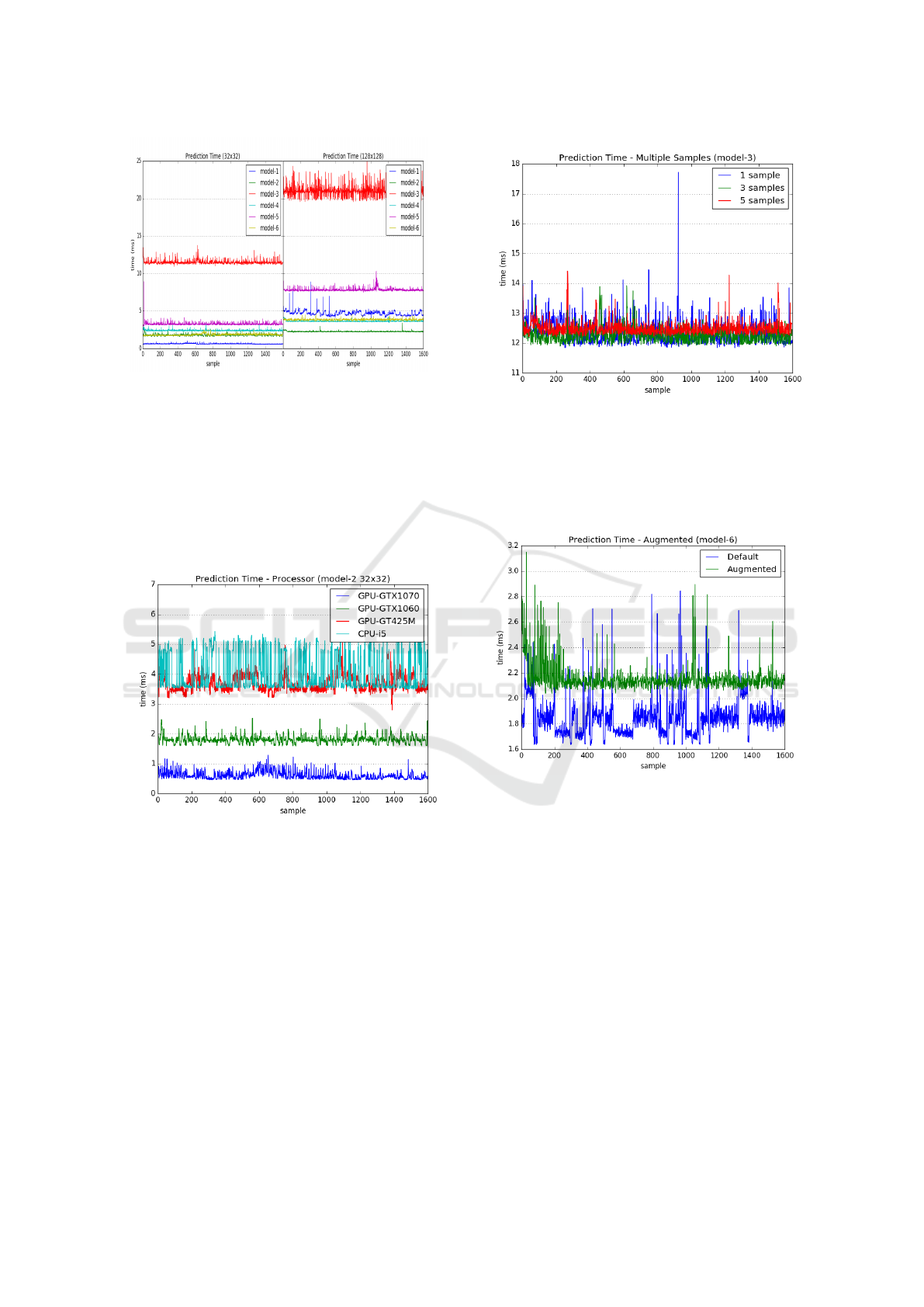
Figure 9: Prediction Times - 32x32 pixels against 128x128

pixels.

the results for prediction times measured on 4 differ-

ent systems. Both a faster and a slower GPU were

used as well a CPU based system for comparison. In

this present work we were not able to perform mea-

surements with an embedded solution, more applica-

ble in a real-time system, which will have to be left

for future work.

Figure 10: Prediction Times per Processor.

Considering that in a real-time application for

trafﬁc sign classiﬁcation, one particular frame from

the video stream can contain multiple detected signs,

which can be fed to the classiﬁcation algorithm all

at once for possible improved performance. Another

experiment was performed where multiple samples

were trained for comparison and the graph in Fig. 11

shows that the overall performance was not affected

by the number of samples to be predicted at the same

time. We tested with 1, 3 and 5 samples. The time in

the graph represents the average time per sample and

the behavior was conﬁrmed by similar data collected

from other trained models.

A ﬁnal experiment was performed using the

trained models with the augmented dataset in order

Figure 11: Prediction Times for Multiple Samples.

to determine if the larger dataset (that gave us better

accuracy) would affect the overall classiﬁcation time.

Fig. 12 shows an increase of about 16% in prediction

time for a dataset 5 times larger than the original.

Figure 12: Prediction Times for Augmented Dataset.

8 CONCLUSION

Even though the primary goal for this project was

not to achieve the best possible accuracy, we were

able to obtain satisfactory results bordering the 99%

mark, with slightly better numbers for the augmented

dataset. About the prediction time results, when we

combine all the performed experiments together, the

best observation we can make is, the average time for

classiﬁcation is somewhat proportional to the number

of convolutional layers in the respective model. On

the contrary, results are not necessarily proportional

to the actual total number of layers in the model or

even the number of parameters in the model. Over-

all, the choice of a particular convolutional model

plays a bigger role than the change in image size or

VEHITS 2017 - 3rd International Conference on Vehicle Technology and Intelligent Transport Systems

266

an augmentation of the dataset. Also, when com-

paring prediction times for a single sample versus

multiple samples, we saw no differences at all, giv-

ing the possibility of parallel classiﬁcation of multi-

ple signs per video frame, instead of just one sign.

In all cases, the data collected is hardware dependent,

as demonstrated, but with the current state-of-the-art

GPUs, real-time capability is indeed achievable, even

though, from our experiments, some of the deepest

models did not show fast enough results, especially

when we consider the fact that we are simply talk-

ing about classiﬁcation time and not account for the

actual trafﬁc sign localization within the video frame

captured. Several different processors ran six differ-

ent CNN Deep Learning models. The models were

trained and veriﬁed to identify German trafﬁc sign

images with varying orientations and augmentations

from the GTSRB benchmark dataset with a high ac-

curacy. With some variations to the dataset, identiﬁ-

cation of images occurred in less than one millisec-

ond on one of the processors. In others cases, with

deeper networks, more speciﬁcally with multiple con-

volutional layers, the results were not as good in com-

parison with shallower networks along with a depen-

dency on the processor used. Our model 6 has just

three convolutional layers and it gave the best accu-

racy. After a certain depth, the features that the net-

work looks for may not make sense for the classiﬁ-

cation purposes and we believe this could possibly be

one of the reasons for the multiple convolutional lay-

ers not performing better. We aim to further improve

prevention of gradient vanishing and use deep resid-

ual learning with deeper networks to observe their be-

havior. As future work, we can modify the dataset

by converting the images to gray-scale, known to be

helpful to improve accuracy as it was the case with the

winner in the GTSRB competition. Another aspect to

consider is the distribution of the images within the

classes which are not homogeneous. Most common

trafﬁc signs have up to 3 thousand images, while the

least common ones have only a few hundred. In this

case, a reduced version of the dataset, by removing

classes where the number of images is less than 1000,

could give us a more homogeneous dataset, and hope-

fully an increase in overall accuracy, by not relying

on classes with too few trained samples. And yet an-

other aspect to be considered is to ﬁne-tune the mod-

els used in the experiment, in terms of activation and

loss functions and its parameters. In terms of hard-

ware, this experiment was limited to desktop or note-

book PCs, and so, it did not consider some of the em-

bedded platforms that are intended to real-time appli-

cations like trafﬁc sign classiﬁcation. We intend to

implement these networks on NVDIA Tegra X1 de-

velopment board and achieve great increment in the

classiﬁcation speed for real-time applications.

REFERENCES

Bojarski, M., Del Testa, D., Dworakowski, D., Firner, B.,

Flepp, B., Goyal, P., Jackel, L. D., Monfort, M.,

Muller, U., and Zhang, J. e. a. (2017). End to end

learning for self-driving cars. Arxiv.org.

Chen, L., Li, Q., Li, M., Zhang, L., and Mao, Q. (2012). De-

sign of a multi-sensor cooperation travel environment

perception system for autonomous vehicle. Sensors,

12(12):12386–12404.

Ciresan, D., Meier, U., Masci, J., and Schmidhuber, J.

(2011). A committee of neural networks for trafﬁc

sign classiﬁcation. The 2011 International Joint Con-

ference on Neural Networks.

Greenhalgh, JackMirmehdi, M. (2012). Real-time de-

tection and recognition of road trafﬁc signs. IEEE

Transactions on Intelligent Transportation Systems,

13(4):1498–1506.

Igel, C. German trafﬁc sign recognition

benchmark gtsrb dataset available at:

http://benchmark.ini.rub.de/?section=home.

Jin, J., Fu, K., and Zhang, C. (2014). Trafﬁc sign recogni-

tion with hinge loss trained convolutional neural net-

works. IEEE Transactions on Intelligent Transporta-

tion Systems, 15(5):1991–2000.

Le, T. T., Tran, S. T., Mita, S., and Nguyen, T. D. (2010).

Real time trafﬁc sign detection using color and shape-

based features. Intelligent Information and Database

Systems, pages 268–278.

Mao, X., Hijazi, S., Casas, R., Kaul, P., Kumar, R., and

Rowen, C. (2016). Hierarchical cnn for trafﬁc sign

recognition. 2016 IEEE Intelligent Vehicles Sympo-

sium (IV).

Menge, Anheuser-Busch, O. (2016). Complete ﬁrst self-

driving truck delivery of beer. Neural Networks.

Sermanet, PierreLeCun, Y. (2011). Trafﬁc sign recognition

with multi-scale convolutional networks. The 2011

International Joint Conference on Neural Networks.

Stallkamp, J., Schlipsing, M., Salmen, J., and Igel, C.

(2012). Man vs. computer: Benchmarking machine

learning algorithms for trafﬁc sign recognition. Neu-

ral Networks, 32:323–332.

Trivedi, M. M. Lisa dataset. available at:

http://cvrr.ucsd.edu. Cvrr.ucsd.edu.

Zeng, Y., Xu, X., Fang, Y., and Zhao, K. (2015). Trafﬁc

sign recognition using deep convolutional networks

and extreme learning machine. Lecture Notes in Com-

puter Science, pages 272–280.

Empirical Evaluation of Convolutional Neural Networks Prediction Time in Classifying German Trafﬁc Signs

267