Models for Predicting the Development of Insulin Resistance

Thomas Forstner

1,*

, Christiane Dienhart

, Ludmilla Kedenko

, Gernot Wolkersdörfer

and Bernhard Paulweber

Department of Applied Systems Research and Statistics, Johannes Kepler University Linz,

Altenberger Strasse 69, 4040 Linz, Austria

Department of Internal Medicine I, Paracelsus Medical University/Salzburger Landeskliniken,

Muellner Hauptstrasse 48, 5020 Salzburg, Austria

Keywords: Predictive Models, Insulin Resistance, Logistic Regression, ROC Analysis.

Abstract: Insulin resistance is the leading cause for developing type 2 diabetes. Early determination of insulin

resistance and herewith of impending type 2 diabetes could help to establish sooner preventive measures or

even therapies. However, an optimal predictive model for developing insulin resistance has not been

established yet. Based on the data of an Austrian cohort study (SAPHIR study) various predictive models

were calculated and compared to each other. For developing predictive models logistic regression models

were used. For finding an optimal cut-off value an ROC approach was used. Based on various biochemical

parameters an overall percentage of around 82% correct classifications could be achieved.

1 INTRODUCTION

Insulin resistance (IR) is a condition in which,

muscle, fat and liver cells do not respond properly to

insulin and these cells therefore cannot easily absorb

glucose from the bloodstream. So, the body needs

higher levels of insulin to help glucose enter the

cells and as consequence the so called beta cells in

the pancreas subsequently increase their production

of insulin to try to keep up with this increased

demand for insulin by producing more insulin. As

long as the beta cells are able to produce enough

insulin to overcome the insulin resistance of the

cells, blood glucose levels stay in a healthy range.

But over time the beta cells fail to keep up with the

body's increased need for insulin and without

enough insulin, excess glucose builds up in the

bloodstream. This can lead to diabetes and other

serious health disorders (Rutter et al., 2008).

Diabetes is often asymptomatic and around 50%

of patients suffering from type 2 diabetes are

undiagnosed and the delay from disease onset to

diagnosis can exceed 10 years. At the time patients

are diagnosed around 25% have established

retinopathy and around 50% have signs of diabetic

tissue damage (Griffin et al., 2000). Furthermore

type 2 diabetes is affecting around 8% of the current

global adult population and the prevalence is

growing worldwide (Keating, 2015).

Early determination of insulin resistance and

herewith of impending type 2 diabetes could help to

establish sooner preventive measures or even

therapies.

The gold-standard for quantifying insulin

resistance is the hyperinsulinemic euglycemic clamp

but this impractical in epidemiological studies

because the measurement takes about two hours and

medical attention is needed. Therefore a commonly

used surrogate endpoint is the homeostatic model

assessment (HOMA) which is derived from the

product of fasting glucose and insulin levels.

The HOMA index is a robust tool for the

assessment of insulin resistance in epidemiological

studies. HOMA index values larger 2.0 are used as an

indication for insulin resistance (Griffin et al., 2000).

The aim of this work was to develop a predictive

model for insulin resistance based on various clinical

parameters and to evaluate this model based on an

ROC approach.

2 DATA

As study population the data of an Austrian cohort

study (SAPHIR study, Salzburg Atherosclerosis

Prevention program in subjects at High Individual

Risk) was used.

Forstner, T., Dienhart, C., Kedenko, L., Wolkersdörfer, G. and Paulweber, B.

Models for Predicting the Development of Insulin Resistance.

DOI: 10.5220/0006344801210125

In Proceedings of the 6th International Conference on Data Science, Technology and Applications (DATA 2017), pages 121-125

ISBN: 978-989-758-255-4

121

The prospective SAPHIR study was conducted

from 1999 to 2002 and involved unrelated male and

female subjects between 40 and 70 years, who lived

in the greater Salzburg region and responded to

invitations by their family or workplace physician or

to announcement in the local press. The study has

been approved by the ethical committee of Salzburg

and written consent was granted by the participants.

At baseline and after approximately 3 years the

participants were subjected to a screening program

that included a personal and family history and a

physical examination. These evaluations also

included a panel of laboratory tests, measurement of

visceral fat mass, body composition, insulin

sensitivity, intima-media thickness of the carotid

arteries and a detailed medical history. HOMA

indices have been used to define the level of insulin

sensitivity.

In total, 1,770 subjects were included in the

SAPHIR study. All subjects of the SAPHIR study

were invited to a second follow-up examination 5

years after their completion of the SAPHIR study.

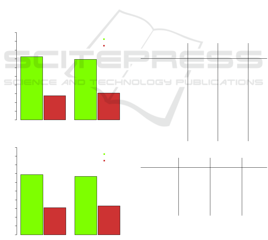
Figure 1: Insulin resistance, SAPHIR study population.

Figure 2: Insulin resistance, complete case population.

This resulted in a response of 1386 subjects,

which were used for the model building process.

Because of missing data only 480 (“complete case

population”) of these 1386 subjects could be used.

The distribution of insulin resistance was similar

between the two populations. The largest difference

was 3.4 percent points. Subjects with insulin

resistance at baseline were also included into the

model because in “real life” the status of insulin

resistance of the subject at baseline is unknown, so

exclusion would lead to a potential bias

3 PREDICTIVE MODELS

3.1 Approach

Because of the binary nature of the data a logistic

regression approach was chosen to predict the target

variable “indication of insulin resistance at follow-

up”. The baseline covariates there chosen from a

clinical point of view.

Table 1: Continuous baseline covariates.

Baseline covariates

No IR

(mean ± SD)

p-value

2hr-OGTT glucose level

[ /dl]

32.38 ± 28.98 81.47 ± 64.68 <0.001

Adiponectin [µg/ml]

9.19 ± 4.74 6.94 ± 3.67 <0.001

Age [years]

51.06 ± 6.08 52.26 ± 5.72 0.001

BMI [kg/m²]

25.55 ± 3.33 30.09 ± 4.20 <0.001

Fat mass [kg]

16.82 ± 7.8 25.13 ± 9.26 <0.001

F-Insulin [µU/ml]

5.14 ± 1.82 13.53 ± 5.98 <0.001

Glucose [mg/dl]

89.17 ± 8.79 104.91 ± 27.71 <0.001

HbA1c [%]

5.53 ± 0.30 5.87 ± 0.86 <0.001

HDL cholesterol [mg/dl]

62.73 ± 15.71 51.43 ± 12.37 <0.001

HOMA-Index

1.14 ± 0.42 3.53 ± 1.97 <0.001

kITT-Index

4.51 ± 1.20 3.24 ± 1.17 <0.001

Lean mass [kg]

59.35 ± 11.65 64 ± 12.96 <0.001

Triglyceride [mmol/]

108.7 ± 74.21 168.27 ± 102.39 <0.001

Waist-Hip-Ratio

0.88 ± 0.08 0.93 ± 0.07 <0.001

Table 2: Categorical baseline covariates.

Baseline covariates

No IR

(%, n)

p-value

Gender

female

male

476 (72.8%)

795 (72.1%)

178 (27.2%)

307 (27.9%)

0.783

Hypertension

yes

789 (80.8%)

457 (62.0%)

188 (19.2%)

280 (38.0%)

<0.001

Incident diabetes

yes

1261 (75.0%)

10 (13.5%)

421 (25.0%)

64 (86.5%)

<0.001

Hypertension was defined as a systolic blood

pressure above 130 mmHg and a diastolic blood

pressure above 85 mmHg. In the early stages of

diabetes sometimes no insulin resistance has

Insulin Resistance - SAHPIR Study Population

Valid %

0 102030405060708090100

72.4% (n=1271)

27.6% (n=485)

69.4% (n=946)

30.6% (n=418)

YES

Baseline Follow-Up

Insulin Resistance - Complete Case Population

Valid %

0 102030405060708090100

69.0% (n=331)

31.0% (n=149)

66.9% (n=321)

33.1% (n=159)

YES

Baseline Follow-Up

DATA 2017 - 6th International Conference on Data Science, Technology and Applications

122

developed yet, therefore baseline incident diabetes

was also included as a covariate in the model.

Incident diabetes was defined as a fasting plasma

glucose level ≥ 126 mg/dl, a 2-hr OGTT glucose of

≥ 200 mg/dl or current use of hypoglycaemic drug

therapy regardless the reason.

Continuous data was compared between the two

groups using the two sample independent t-test in

case of normality (verification with the

Kolmogorov-Smirnov test with Lilliefors correction)

and variance homogeneity (verification with the

Levene test). If continuous data was normally

distributed but variance was heterogeneous Welch’s

t-test was used and if data showed no normal

distribution, the Mann-Whitney-U test was used.

Unpaired categorical data was compared using

Fisher´s exact test. For calculations SPSS (IBM

Corp. Released 2013. IBM SPSS Statistics for

Windows, Version 22.0. Armonk, NY: IBM Corp.)

and the statistical computing software R Version

3.2.3 (R Foundation for Statistical Computing,

Vienna, Austria. URL http://www.R-project.org)

were used. The uncorrected type I error was set at

5% (two-sided), this means no adjustment for the

type I error was made.

3.2 First Model

The a-priori selected baseline covariates (except

gender) discriminated very well regarding the

indication of baseline insulin resistance, so for a first

model all baseline covariates were used to predict

indication of insulin resistance at follow-up.

The estimates based on this logistic regression

model (model Ia) are presented in the table below.

Table 3: Variables of the model Ia.

Baseline Covariates p-value Odds-Ratio 95% CI for OR

2hr-OGTT glucose level [mg/dl] 0.001

1.015 1.006-1.024

Adiponectin [µg/ml] 0.038

0.911 0.834-0.995

Age [years] 0.547 0.983 0.931-1.039

BMI [kg/m²] 0.077 1.169 0.983-1.39

Fat mass [kg] 0.407 0.972 0.91-1.039

F-Insulin [µU/ml] 0.001

1.706 1.24-2.348

Glucose [mg/dl] 0.011

1.058 1.013-1.106

HbA1c [%] 0.977 0.986 0.397-2.452

HDL cholesterol [mg/dl] 0.010

0.963 0.936-0.991

HOMA-Index 0.008

0.212 0.067-0.672

kITT-Index 0.893 1.017 0.794-1.303

Lean mass [kg] 0.980 1.000 0.951-1.051

Triglyceride [mmol/] 0.979 1.000 0.996-1.004

Waist-Hip-Ratio 0.394 9.645 0.052-1773.282

Gender (male vs. female) 0.037

3.886 1.086-13.897

Hypertension (no vs. yes) 0.395 0.776 0.432-1.393

Incident diabetes (no vs. yes) 0.708 1.403 0.238-8.265

Constant 0.004

0.000 1.006-1.024

This model yielded an overall percentage of

82.2% correct classifications (90.5% correct

classifications for no indication of insulin resistance

and 65.3% correct classifications for indication of

insulin resistance). A Nagelkerke’s R² of 0.550

indicated also a good model fit.

Based on the model an increase in one unit of

“2hr-OGTT glucose level [mg/dl]”, “F-Insulin

[µU/ml]” and “Glucose [mg/dl]” is associated with a

significant higher chance for insulin resistance. An

increase of one unit in “Adiponectin [µg/ml]” and

“HDL cholesterol [mg/dl]” is associated with a

significant lower chance for insulin resistance. There

was also a significant increased chance for women

suffering from insulin resistance at follow-up.

Interestingly low levels of HOMA-index

baseline were associated with a higher chance of

insulin resistance at follow-up (Odds Ratio = 0.212).

But a univariate analysis yielded the expected

association (Odds Ratio = 4.315, p < 0.001**). So

this unexpected multivariate Odds Ratio may be

caused through the multicollinearity of the model.

The confidence interval of the “Waist-Hip-

Ratio” was extremely large so a bootstrapping

approach based on 1000 bootstrap-samples was used

to validate the numerical integrity of model Ia. The

confidence interval for “Waist-Hip-Ratio” was even

more extreme so this variable was excluded from the

model. The results from this model (model Ib)

remained almost the same like model Ia.

The classification results of the model Ib are

presented in the table below.

Table 4: Classification result of model Ib.

Predicted

Observed

no IR IR

% correct

no IR

272 29 90.4

51 97 65.5

Overall %

82.2

(Cut-Off value 0.5)

3.3 Second Model

The first model yielded a good overall percentage of

correct classification results but was relatively

complex because various laboratory parameters were

needed. So the next step was to reduce the

complexity of the model using a variable selection

approach (Bursac et al., 2008). A reduced model

with similar results but fewer needed laboratory

parameters would also be more cost efficient.

The first approach was using a backwards-

likelihood-ratio-approach (probability for entry 0.05,

probability for removal 0.10) which led to an overall

percentage of correct classification of 81.7% but this

Models for Predicting the Development of Insulin Resistance

123

model was again relatively complex (8 covariates

were selected). So the next step was using a

forwards-likelihood-ratio-approach (probability for

entry 0.05, probability for removal 0.10) which

resulted in a similar overall percentage of correct

classifications but with a reduced number of

covariates.

The estimates based on this forward-logistic

regression model (model II) are presented in the

table below.

Table 5: Variables of the model II.

Baseline Covariates p-value Odds-Ratio 95% CI for OR

2hr-OGTT glucose level [mg/dl] 0.001

1.013 1.005-1.021

Adiponectin [µg/ml] 0.012

0.900 0.83-0.977

BMI [kg/m²] 0.002

1.123 1.044-1.207

F-Insulin [µU/ml] <0.001

1.188 1.095-1.289

HDL cholesterol [mg/dl] 0.001

0.959 0.936-0.982

Gender (male vs. female) 0.005

2.599 1.337-5.052

Constant 0.001

0.019 1.005-1.021

The result was a relatively compact model with an

overall percentage of 81.9% correct classifications

(91.6% correct classifications for no indication of

insulin resistance and 62.3% correct classifications for

indication of insulin resistance). A Nagelkerke’s R² of

0.531 indicated again a good model fit.

Based on this model an increase in one unit of

“2hr-OGTT glucose level [mg/dl]”, “BMI [kg/m²]”

and one unit of “F-Insulin [µU/ml]” is associated with

a significant higher chance for insulin resistance.

An increase in one unit of “Adiponectin

[µg/ml]” and one unit of “HDL cholesterol [mg/dl]”

is associated with a significant lower chance for

insulin resistance. There was also a significant

increased chance for women suffering from insulin

resistance at follow-up.

The robustness of this model was again verified

with a bootstrapping approach based on 1000

bootstrap-samples; no inconsistency was detected.

Compared to the overall percentage of correct

classifications and correct classifications for no

indication of insulin resistance the percentage of

correct classifications for indication of insulin

resistance was low. So based on a Receiver

Operating Characteristic curve (ROC curve) an

optimal cut-off value for the predicted probabilities

was searched.

4 ROC ANALYSIS

A standard technique for summarizing the

performance of a predictive model over a range of

cut-off-values is the Receiver Operating

Characteristic curve (ROC curve) (Sweets, 1988).

Since the ROC curve summarizes the predictive

power of a model over all possible cut-off-values, it

is more informative than a simple classification table

for a fixed cut-off value.

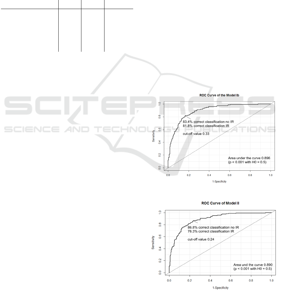
The area under the curve (AUC) can be used as a

performance metric for ROC curves. A higher area

under the curve indicates a better prediction power.

The previous logistic regression models yielded an

area under the curve of 0.896 (model Ib)

respectively 0.890 (model II).

For the previous logistic regression models the

standard cut-off-value of 0.5 was used for the

predicted probabilities. To maximize the

effectiveness of a predictive model the cut-off value

can be varied to achieve a higher true positive rate

(“sensitivity”) and a higher true negative rate

(“specificity”). The Youden index method (Youden,

1950) was used to the define the optimal cut-off

value for the two models.

The idea of the Youden index is to maximize the

difference between true positive rate and false

positive rate (“1 – specificity”). This means in other

words that the Youden index is specified as the point

Figure 3: ROC curve for model Ib.

Figure 4: ROC curve for model II.

DATA 2017 - 6th International Conference on Data Science, Technology and Applications

124

on the ROC curve which has the largest distance

from the diagonal line. Based on the Youden index

an optimal cut-off-value of 0.33 (model Ib)

respectively 0.24 (model II) could be found.

In other papers an achieved area under the curve

of 0.71 (Chiang et al., 2011) or 0.75 (Behboudi-

Gandevani et al., 2016) was reported. In (Er et al.,

2016) various models for predicting insulin

resistance with an achieved area under the curve

from 0.31 up to 0.80 were reported. So the area

under the curve of the two presented predictive

models indicates a slightly better performance.

5 CONCLUSIONS

Based on the data of an Austrian cohort study a

predictive model with an overall percentage of

81.9% correct classifications for predicting insulin

resistance based on gender and 5 biochemical

parameters could be developed. Furthermore the

classification cut-off-value was optimized by the use

of ROC curves to achieve 86.6% correct

classifications for no indication of insulin resistance

and 76.3% correct classifications for indication of

insulin resistance. Additionally based on the R

package “caret” (Kuhn, 2008) a random forest

approach was used for predicting insulin resistance.

This approach yielded a similar overall percentage

(79.2%) of correct classifications (86.6% correct

classifications for no indication of insulin resistance

and 64.2% correct classifications for indication of

insulin resistance).

Limitations of this model are that the data was

collected in a relatively small area and that because

of various missing values in the baseline covariates

and target variable only around 480 of 1386 patients

could be included in the model building process. To

account for this relatively large percentage of

missing values a multiple imputation approach (5

imputations, fully conditional specification method

based on an iterative Markov chain Monte Carlo

algorithm) was used. The results of this approach

yielded very similar results except that the influence

of the covariate gender was not significant anymore

(Odds Ratio = 0.997; p = 0.989) like the univariate

test of gender between baseline insulin resistance.

REFERENCES

Behboudi-Gandevani S., Tehrani F. R., Cheraghi L., Azizi

F., 2016. Could “a body shape index” and “waist to

height ratio” predict insulin resistance and metabolic

syndrome in polycystic ovary syndrome. European

Journal of Obstetrics & Gynecology and Reproductive

Biology, 205: 110-114.

Bursac Z., Gauss C. H., Williams D. K., Hosmer D. W.,

2008. Purposeful selection of variables in logistic

regression. Source Code for Biology and Medicine,

17(3).

Chiang J. K., Lai N. S., Chang J. K., Koo M., 2011.

Predicting insulin resistance using the triglyceride-to-

high-density lipoprotein cholesterol ratio in Taiwanese

adults. Cardiovascular Diabetology, 10(93).

Er L. K., Wu S., Chou H. H., Hsu L. A., Teng M. S., Sun

Y. C., Ko Y. L., 2016. Triglyceride Glucose-Body

Mass Index Is a Simple and Clinically Useful

Surrogate Marker for Insulin Resistance in

Nondiabetic Individuals. PLoS ONE, 11(3).

Griffin S. J., Little P. S., Hales C. N., Kinmonth A. L.,

Wareham N.J., 2000. Diabetes risk score: towards

earlier detection of type 2 diabetes in general practice.

Diabetes/Metabolism Research and Reviews, 16(3):

164-171.

Keating B, J., 2015. Advances in Risk Prediction of Type

2 Diabetes: Integrating Genetic Scores with

Framingham Risk Models. Diabetes, 64(5):1495-1497.

Kuhn M., 2008. Building predictive models in R using the

caret package. Journal of Statistical Software, 28(5):

1-26.

Rutter M. K., Wilson P. W. F, Sullivan L. M., Fox C. S.,

D’Agostino R. B., Meigs J. B., 2008. Use of

Alternative Thresholds Defining Insulin Resistance to

Predict Incident Type 2 Diabetes Mellitus and

Cardiovascular Disease. Circulation, 117(8):1003-

1009.

Sweets J. A., 1988. Measuring the accuracy of diagnostic

systems. Science, 240:1285–1293.

Youden W. J., 1950. Index for Rating Diagnostic Tests.

Cancer, 32-35.

Models for Predicting the Development of Insulin Resistance

125