
Robust PI
D
, H
and Smith Predictor Controller Design for
Time Delay Systems
Youcef Zennir, Mohand Said Larabi and Hamza Zemaili
Automatic Laboratory of Skikda, Skikda University, 26 route el-hadaiek, Skikda, Algeria
Keywords: Robust Control, Fractional Order Controller, Smith Predictor Controller, H
Controller, Identification,
Industrial System, System with Time Delay.
Abstract: This paper present optimal robust control with different controllers design used in the industrial (didactic or
process) system. We designed a controller base on Smith's predicator controller and Fractional order PID
(PI
D
) controller and H
∞
controller. These control techniques has been used with different controller’s
types to ensure an optimum control in term of dynamic and static performances of a complex didactic
industrial process in accordance with the required specifications. We have described in more details the
process, the mathematical model, the structure of FOPID controller and the approximation method
(singularity function method of Charef) used to approximate fractional order. The principle of control is
decried as well with the different types of controllers used in this study. Finally several simulation and real
results are presented which have proved the efficiency of this new control design in term of: stability,
robustness and precision.
1 INTRODUCTION
To be robust, an industrial process must be well
controlled. Indeed, competitiveness requires keeping
process values as close as possible to its required
optimum performance and process conditions: such
as the products quality, production flexibility,
energy saving and safety of personnel, facilities and
the environment. The main role of industrial
controller is to keep the process under control with
the guarantee of a good dynamic and static
behaviour performance. Which can be achieved by
adjusting and adapting the transfer function
parameters in order to as close as possible to the real
process? In general, an industrial process is
modelled by a non-linear, linear (after linearization)
or linear mathematical model with a time delay
(Boyd, 1991). Regardless if these models are stable
or not are required a controller (control action) to
ensure the desired performance. The objective of
automatic regulation or servo-control of a process is
to keep the process values as close as possible to its
optimum of operating points, predefined by the
process specification (imposed conditions or
performance). Safety aspects of staff and facilities
should be taken into accounts, such as those relating
to energy and respect for the environment. The
specifications define qualitative criteria to be
imposed, which are usually translated by
quantitative criteria, such as stability, precision,
speed or evolution laws. Before going ahead and
develop the controller architecture and structure and
in case of unknown process parameters, an
identification phase is mandatory. Different methods
of identification exist in the literature (Broida,
Strejc, etc.) (Boyd, 1991; Ljung, 1999; Barraud
2006), in our study we have used Ident a Matlab
identifications toolbox function and we did a study
of a flow control system (Figure 4) by computing its
mathematical model (Abraham, 2015) via applying a
different identification methods (Broida, Strejc, etc.)
and synthesis of its control laws using several types:
FOPID, Smith predictor and H
controllers
(Barraud, 2006), and then at the end we checked the
simulation results with the process experiments.
2 CONTROLLERS DESIGN
In the literature, it exist a large number of linear or
discrete linear controllers adequate to control an
industrial process which have a linear system
Zennir, Y., Larabi, M. and Zemaili, H.
Robust PI
λ
D
µ
, H
∞
and Smith Predictor Controller Design for Time Delay Systems.
DOI: 10.5220/0006399805430550
In Proceedings of the 14th International Conference on Informatics in Control, Automation and Robotics (ICINCO 2017) - Volume 1, pages 543-550
ISBN: 978-989-758-263-9
Copyright © 2017 by SCITEPRESS – Science and Technology Publications, Lda. All rights reserved
543
behavior (Kumar, 2014). Among the most common
and most used controllers are PI, PD and PID
different structures (Shamsuzzoha 2008). Also, there
is another type of controller which is more robust
than the Standart PID such as the Fractional order
PID controller (FOPID) (Bettou, 2008; Bouras,
2013; Djari, 2014). Other types of controllers are
developed specifically to control the systems with
time delay such as Smith's predictor. This controller
was proposed for the first time by OJ Smith in 1957
(Esmaeilzade, 2014).The main idea behind Smith's
predictor is that, since it is well known to correct
systems without time delay with a corrector (PID for
example) (Aidan, 1996; Resceanu, 2009). It does not
correct the system without delay but the output will
then be estimated by delaying it by the value of the
time delay of the system. This very simple approach
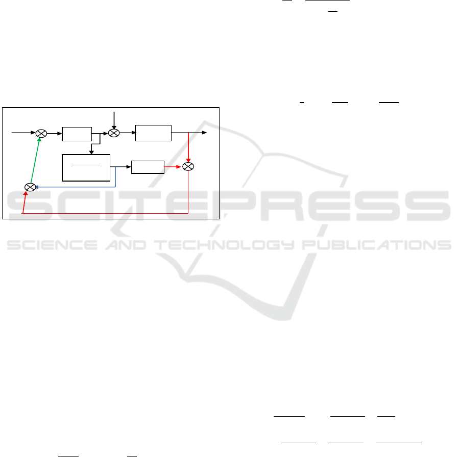
leads to the following structure:
Figure 1: Structure of Smith Predictor ( L=Td; Ks=Kp;
=Td).
Different structures of Smith predictor has been
proposed in literature with different controllers. Note
that, the implementation of a Smith predictor
controller needs a very good model of the process.
In our study we have used only Fractional order PID
(FOPID) controller and with Smith predictor. The
structure type of the FOPID controllers is Fractional
order controller: PI
λ
D
. In control theory, the
conclusion about fractional control system is that it
can increase the stability region and robustness
(Esmaeilzade, 2014) moreover it gives performances
at least as good as its integer counterpart (Grimble,
2006). The transfer function of a FOPID controller,
which was initially proposed by Podlubny in 1999
(Esmaeilzade, 2014), is given by:
1
,
,0
(1)
Where Kp, KI, KD R and , R+: are the
controller tuning parameters and the controller
design problem is to determine the suitable values of
these unknown parameters in such way it responds
to all control objectives (Grimble, 2006). Many
methods in literature have been proposed for FOPID
approximation (Bouras, 2013). In this work we have
used singularity function approximation method of
Charef (Bettou, 2011), applied in FOPID controller.
The fractional-order integrator
,
∈
R+ is
approximated as:
1
≅
1
,
01,
∈
(2)
To have a good tuning parameters of the PI
D (Kc,
Ti, ) we have used the following algorithm
(Bouras, 2013) described in the steps below:
Step1: calculate the parameters
i
for 0≪i≪2
∙
∙
(3)
u
: the unit magnitude frequency of reference
model;
m: the derivation fractional order of the reference
model;
i
: calculated with the reference model parameters.
Step 2: calculate the parameters y
i
for 0≪i≪2
Using the following formulas:
∙
(4)
∙
∙
(5)
∙
∙
(6)
With y
i
: calculated from the transfer function Gp(s)
compared to the variable s at the point ωu; N :
samples number.
Step 3: calculate the parameters X
i
for 0 ≪i≪2
As per the following formulas:
.
(7)
.
.
.
(8)
With X
i
: derived from the controller transfer function
C(s).
Step 4: calculate the parameters K
c
, T
i
, with the
following formulas:
C(s)
tf4(s)
e
-Ls
1
∙
r
u
y
d
Process
e
p
y
a
+
-
+
+
-
+
ICINCO 2017 - 14th International Conference on Informatics in Control, Automation and Robotics
544
.
1
.
(9)
.
(10)
3 OPTIMAL CONTROL WITH H
Several representations are possible to solve the
control problems of the closed loop system, such as
H
∞
and H
2
optimization. Therefore it is practical to
have a general formula, in order to have a "standard
problem" for this type of control. The configuration
of the closed loop system with the various
specifications (weighting functions) is shown in
Figure (2).
Figure 2: Problem formulation Standard.
Where: W
t
(s): transfer matrix of the stability
specification; W
a
(s): transfer matrix relating to the
additive error; W
p
(s): matrix for transferring the
performance specification.
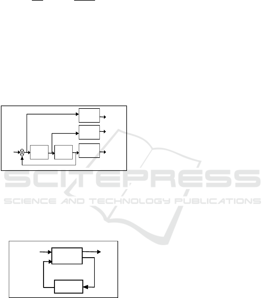
The general configuration of the standard
problem (Tsai, 2014) is presented in Fig.7 (LFT,
Linear Fractional Transformations representation).
Figure 3: Standard problem (LFT representation).
Where: u: system commands (dimension "m");
w: disturbance inputs (dimension "l");
y: measurements on the system (outputs)
(dimension "q");
z: controlled outputs (dimension "p"); x: state vector
(dimension "n")
The solution of the standard problem
(generalized mixed sensitivity problem) is found by
computing a control law u - delivered by a controller
K(s) - such that: u = K(s).y minimizing the influence
of the perturbation signal w on the output signal z,
namely:
∞
1
(11)
With:
T(s): Complementary Sensitivity defined by
(12)
L(s): is the Open loop L(s) = G(s) K(s)
R(s): Transfer to Control defined by
(13)
S(s): Sensitivity defined by:
(14)
We have associated with the standard problem the
following cost function T
zw
:
(15)
With:
(16)
(17)
And we have illustrated the steps for obtaining the
K(s) controller parameters by solving the problem
H
∞
. The problem of optimization by H
∞
is to find a
controller K(s) which stabilize the process, so as to
minimize the transfer between the inputs w and the
outputs z.
‖
‖
∞
max
(18)
The structure of the central controller K(s) is given
by the following function:
∞
∞
∞
∞
(19)
The association of the sensitivity function S(s) will
improve our controller performance in term of
closed-loop stability and attenuates the resonance
peaks on the maximum singular value of the
sensitivity S(s) (Tsai, 2014). The solution to the
problem of optimization by H∞ mentioned earlier
will be realized by the iteration on the parameter γ
then the optimal robust controller K(s) will have to
satisfy the condition: ||Tzw(jω)||∞ ≤ γ. The
P(s)
K(s)
w
u y
z
K(s) G(s)
w
p
(s)
W
a
(s)
W
t
(s)
Z
1
(s)
Z
2
(s)
Z
3
(s)
u(s)
e(s)
w
+
-
Robust PI
λ
D
µ
, H
∞
and Smith Predictor Controller Design for Time Delay Systems
545
parameter γ has to satisfy the compromise
"Stability/Performance". The different steps for the
robust controller’s determination are described as
follow. All these calculations steps can be
considered long before obtaining controller
structure, because they must be carried out for each
value of the parameter γ. Therefore it is preferable to
use a calculation algorithm, which computes the
robust controller parameters quicker with very good
accuracy. The robust controller parameters
algorithm is exposed as below:
1. Choice of specifications W
t
, W
p
and W
a
.
2. Realization of the augmented plant P(s).
3. Take γ = 1, synthesize controller H
∞
.
4. Calculation of the cost function Tzw.
5. If ||T
zw
(jω)||
∞
≤ γ go to 7.
6. Otherwise adjust γ and go to 2.
7. Frequency Evaluation’s and temporal results.
8. If the results are satisfactory go to 10.
9. Otherwise adjust γ and go to 1.
10. End.
The implementation of the controller will be
obtained by MATLAB software’s via Robust
Control Toolbox.
4 DIDACTIC INDUSTRIAL
PROCESS
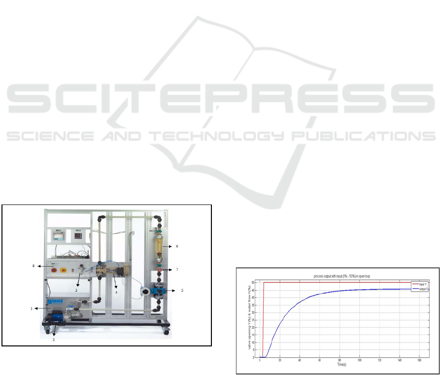
The process illustrated in FIG. 4 consists of
numerous components and accessories (Abraham,
2015). The accessory components are pre-installed
on plates.
Figure 4: Experiment setup of a flow control (Abraham,
2015).
The basic module contains one storage tank: 75L
(1), Centrifugal pump (2), Compressed air controller
with pressure gauge (0-2,5bar) with quick coupling
for supplying experiments (3), orifice with
Differential Pressure Sensor (Electro-pneumatic
control valve) (4), flow Rate Sensor
(Electromagnetic) (5), rotameter (6), valve (7) and
Switch cabinet (8). The Controlled System Flow is
operated with water as the working medium and
consists of a variable area flow meter. The flow
resistance can be configured using a valve (7), which
changes the flow properties in the controlled
systems.
One particular benefit of these controlled
systems is that, thanks to the float, all changes in the
flow rate caused by interference or behaviour of a
controller can be observed directly. The training
system has an electronic sensor with display for
measuring flow rate. It is suitable for measuring
flow rates of liquids in closed tubes. The
measurement variable is the flow rate. The ideal
flow velocity is 1- 3m/s.
The measurement principle is electromagnetic
induction according to Faraday's law.
Electromagnets or coils generate a magnetic field, in
which a conductor moves. This induces a voltage.
Here, the medium flowing in the flow rate sensor
corresponds to the moving conductor. The magnetic
field is generated by pulsed direct current of
alternating polarity. The identification methods used
to identify our process are described in the following
section.
5 PROCESS IDENTIFICATION
The search of an industrial process model is
necessary and must result in a model correctly
representing the behaviour of the process. However,
the model must not be too sophisticated, at the risk
of being incompatible with the available corrector,
or be too simplistic not to mask certain aspects that
are detrimental to proper functioning.
Figure 5: Process step response with input 0 % 50% in
open loop.
ICINCO 2017 - 14th International Conference on Informatics in Control, Automation and Robotics
546
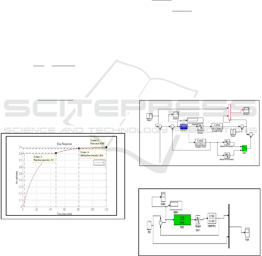
The choice of a model, like its determination,
must be judicious (Liung, 1999). The system can
then be excited by a step signal with different
values. In principle, the output and input must be of
the same type with linear system (figure 5). If not,
the system is nonlinear (Barraud, 2006).
We have used Matlab function: ident from the
identification toolbox. The structure of parametric
estimation method is a simple transfer function in
continuous time that describes a linear dynamic
system. This model is characterized by a static gain,
time constants and time delay. If some parameters
are known, we need just enter their values and tick
the box "Known". The estimation algorithm will use
these values for the model. The behaviour of the
system is close to the first-order systems with a
small time delay, so we start from this principle and
we have made the identification with the four
datasets. The general form of the transfer function is
given by the following formula:
tf
s
Xs
Ys
K
T
∙s1
∙e
∙
(20)
The obtained model with this method is illustrated in
the following formula:
tf
s
0.89686
20.539∙s1
∙e
.∙
(21)
The tf4 is the model that represents better the real
system. The index response of the open-loop model
(tf4) is illustrated in the following figure:
Figure 6: Step response of model tf4 in open loop.
The open loop characteristics are not satisfactory
(the system is very slow, final value different of 1)
(figure 6). Hence the need to used a controller to
ensure the optimal characteristics and improved the
stability of process. In the following section
different controllers used in this study has been
described and on particularly the Smith’s predictor
controller with new structure.
6 SIMULATION
The simulation is done on a closed loop with an step
input. The simulation Parameters are as follows:
FOPID controller: m=0.9; KI =12.3231
H
controller:
= 20.539; System time constant in open loop
a = 10; Acceleration parameter
w
o
= 1/(a*);
∙
: Performances specification
W
2
= [];
.∙
: stability specification
PID controller: kp1=10.5; ki1=0.808; kd1=1.84;
Smith Predictor: Delay1=0.5s and delay2=2.5s;
Disturbance equal 1 at t=40s; Simulation Time
=100s; the simulation is organized as follows:
First study: controlling the system with FOPID
and PID controllers without Smith predictor.
Second study: controlling the system with S
FOPID and PID controllers with Smith predictor.
Finally controlling the system with H robust
controller
The block diagram of the control is as follows:
Figure 7: Block diagram of Smith predictor and FOPID
controller.
Figure 8: Block diagram with FOPID controller.
Robust PI
λ
D
µ
, H
∞
and Smith Predictor Controller Design for Time Delay Systems
547
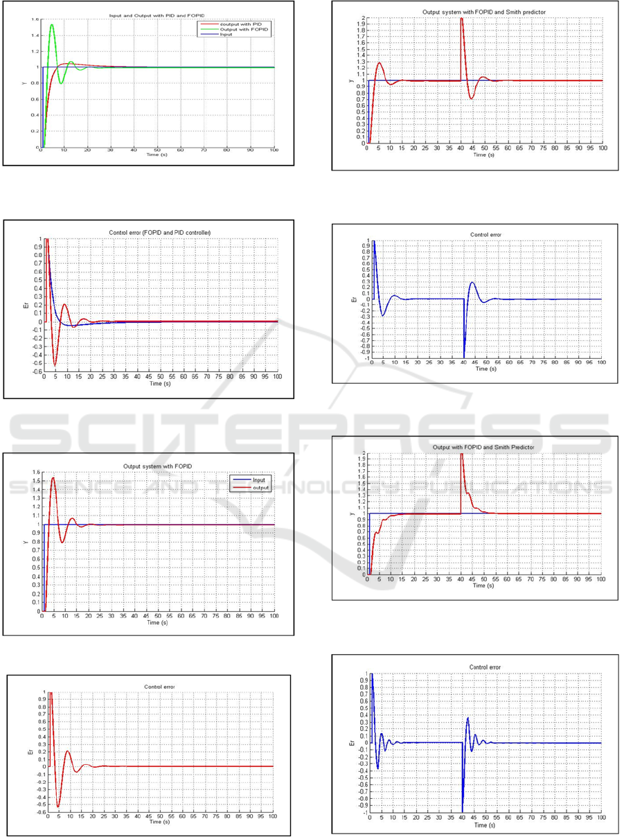
Figure 9: Input and Output curve, with FOPID and PID
controller.
Figure 10: Control error with FOPID (red curve) and PID
controller (bleu curve).
Figure 11: Input and Output curve with FOPID controller.
Figure 12: Control error curve with FOPID controller.
Figure 13: Input and Output curve (Process= model), with
smith Predictor and FOPID controller.
Figure 14: Error control (Process = model), with FOPID
controller.
Figure 15: Input and Output curve (Process model, time
delay=2.5s), with Smith predictor and FOPID controller.
Figure 16: Error control (Process model, time
delay=2.5s), with Smith predictor and FOPID controller.
ICINCO 2017 - 14th International Conference on Informatics in Control, Automation and Robotics
548
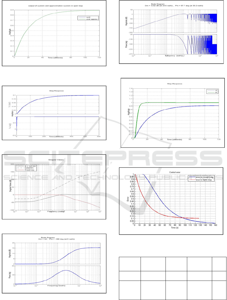
Figure 17: Output of system and approximation system in
open loop.
Figure 18: Output of Z1 and Z3 with (W2=0).
Figure 19: Singular Values.
Figure 20: Frequency response of W3.
Figure 21: Frequency response of disturbances.
Figure 22: Output system curve in open loop (bleu curve)
and in closed loop (green curve).
Figure 23: Control error with H∞ controller.
Table 2: Control error.
Control
error
FOPID
with Smith
Predicto
r
FOPID
PID &
Smith
Predicto
r
H
Process=
model
1.1.10
-6
6.8.
10
-3
6.5.10
-4
3.5.
10
-3
Process
model
(delay
=2.5s)
-9.4.10
-7
8.7.10
-4
The obtained results illustrated in Fig.9 and
Fig.10 show the PID controller is more efficient
Robust PI
λ
D
µ
, H
∞
and Smith Predictor Controller Design for Time Delay Systems
549

(short response time).The Fig.11 until Fig.16
illustrated the efficiency of smith predictor with
FOPID controller with and without disturbance
(very good robustnes, stability and presicion). The
Fig.17 until Fig.23 and Table.III show that the H
∞
controller is more efficient then the FOPID (short
response time and good precision). In the table.III
we can observed that the designed Smith predictor
with FOPID controller gives the best performences
and robustnes.
7 CONCLUSION
In this work we have presented a structure of Smith
Predictor controller based on PID and Fractional
order PID control (FOPID) and robust H
∞
controller
applied to the industrial didactic process, modeled
by a linear model with time delay. A detailed
description of the system was presented with
identification phase. The chosen model has been
validated. the obtained results show the new smith
predictor sutructure with an Fractional order PID
control improves more the performance of the
process compared with PID or H
∞
controller and
keep the study open for further optimization of the
FOPID parameters in case of a big time delay.
Different optimization algorithms can be applied
such as PSO or Genetic algorithms.
REFERENCES
Abraham, D., and Denker, T., 2015. Instruction Manual
RT 450 Modular Process Automation Training
Aidan, O. and John, R., 1996. The control of a process
with time delay by using a modified Smith predictor
compensator. Proceedings of the Irish Conference on
DSP and Control, Trinity College Dublin, pp. 37-44.
Barraud, J., 2006. Control of processes with variable
parameters. Mathematics. E. N.S des Mines de Paris,
p.161.
Bettou, K., 2011. Analyse et réalisation de correcteurs
analogiques d'ordre fractionnaire", Phd-These,
Université de Constantine, p.111.
Bettou, K. Charef, K.A, 2008. A New design method for
fractional PI
λ
D
μ
controller. IJSTA, vol.2(1), pp 414-
429.
Bouras, L. Zennir, Y., and Bourourou, F., 2013. Direct
torque control with SVM based a fractional controller :
Applied to the induction motor. Proceeding of the 3rd
IEEE international conference on system and control,
pp.702-707.
Boyd, S., and Barratt, C., 1991. Linear Controller Design:
Limits of Performance. Originally published by
Prentice-Hall, p.426.
Djari, A., Bouden, T., and Boulkroune, A., 2014. Design
of a fractional order PID controller (FOPID) for a
class of fractional order MIMO systems. J.
Automation & Systems Engineering, vol.8(1), pp. 25-
39.
Esmaeilzade, S.M., Balochian, S., Balochian, H., and
Zhang, Y., 2014. Design of Fractional–order PID
Controllers for Time Delay Systems using Differential
Evolution Algorithm. Indian Journal of Science and
Technology, vol. 7(9), pp.1307–1315.
Grimble, M. J., 2006. Robust Industrial Control Systems:
Optimal approach for polynomial systems. Book,
pp.554.
Kumar, S., and Singh, V.K., 2014. PID controller design
for unstable Processes With time delay. International
journal of innovative research in electrical,
electronics, instrumentation and control engineering,
Vol. 2, Issue 1, pp.837-845.
Kwakernaak, H., 1993. Robust control and H∞
optimization – A tutorial paper. Automatica, Vol. 29
(2), pp. 255-273,
Ljung, L., 1999. System Identification: Theory for the
User. 2
nd
ed. Englewood Cliff, NJ: Prentice Hall.
Reşceanu, F., 2009. New Smith Predictor Structure Used
for the Control of the Quanser SRV-02 Plant. Annals
of the university of Craiova, vol.2.p.7
System. G.U.N.T. Gerätebau, Barsbüttel, Germany,
Version 0.1, p. 215.
Shamsuzzoha, M., and Lee, M., 2008. PID controller
design for integrating processes with time delay.
Korean J. Chem. Eng., vol.25, N° 4, pp.637-645.
Tsai, M., and Gu, D., 2014. Robust and Optimal Control:
A Two-port Framework Approach. Advances in
Industrial Control, Springer, pp.336.
ICINCO 2017 - 14th International Conference on Informatics in Control, Automation and Robotics
550
