A Practical Approach for the Auto-tuning of PD Controllers for Robotic

Manipulators using Particle Swarm Optimization

Ahmed Zidan, Jens Kotlarski and Tobias Ortmaier

Institute of Mechatronic Systems, Leibniz Universit

at Hannover, 30167 Hanover, Germany

Keywords:

Robotic Manipulators, Particle Swarm Optimization, PD Control, Automatic Tuning.

Abstract:

An auto-tuning method of PD controllers for robotic manipulators is proposed. This method suggests a practi-

cal implementation of the particle swarm optimization technique in order to ﬁnd optimal gain values achieving

the best tracking of a predeﬁned position trajectory. For this purpose, The integral of the absolute error IAE is

used as a cost function for the optimization algorithm. The optimization is achieved by performing the desired

movement of the robot iteratively and evaluating the cost function for every iteration. Therefor, the necessary

constraints that guarantee a safe and stable movement of the robot are deﬁned, which are: a maximum joint

torque constraint, a maximum position error constraint and an oscillation constraint. A constraint handling

approach is suggested for the optimization algorithm in order to adapt it to the problem in hand. Finally, the

efﬁciency of the proposed method is veriﬁed through a practical experiment on a real robot.

1 INTRODUCTION

PID control schemes provide simple and effective so-

lutions for most applications of control engineering.

However, the effectiveness of PID controllers is con-

ditioned by accurate tuning of the controller gains.

Robotic manipulators are highly non linear, highly

coupled, Multi-Input Multi-Output (MIMO) dynamic

systems. Using PID controller to control robotic ma-

nipulators can be a desired choice because of its sim-

plicity and effectiveness. However, the conventional

tuning methods of the gains depending on manual or

experimental approaches do not necessarily give sat-

isfactory results for such complex systems (Johnson

and Moradi, 2005).

The difﬁculty of using experimental and manual tun-

ing methods rises in the application ﬁelds, where the

assigned task of a robot might constantly change or

where a robot is of variable conﬁguration or geome-

try (e. g. modular robots). In such cases, the need for

an auto-tuning method is urgent.

Recently, after the rapid increase of computing power,

auto-tuning methods based on optimization tech-

niques has been applied to non linear systems in or-

der to obtain an increased performance with respect

to predeﬁned ﬁtness functions.

In the ﬁeld of robotic manipulators, a number of op-

timization methods (e. g. Genetic Algorithms (GA)

(Kim et al., 2012), Particle Swarm Optimization

(PSO) (Kapoor and Ohri, 2015)) has been used to

automatically tune the PID controllers of robot ma-

nipulators. Also, comparative studies between differ-

ent algorithms have been done in (Ouyang and Pano,

2015) and (Kwok and Sheng, 1994) in order to ﬁnd

the most effective tuning method.

In (Ayala and dos Santos Coelho, 2012), more than

one single objective were considered within the con-

troller design. The proposed optimization method

was based on a multi-objective evolutionary algo-

rithm (MOEA), which aimed to tune the PID con-

troller gains by taking two conﬂicting objective func-

tions into consideration: minimization of position er-

rors and minimization of the control signal variation

(joint torques). In (Pierezan et al., 2014), a com-

parative study between different multi-objective opti-

mization techniques has been introduced and an im-

proved multi-objective particle swarm optimization

(I-MOPSO) has been proposed.

Artiﬁcial intelligence techniques like fuzzy logic and

neural networks have also been implemented to build

PID tuning systems for robotic manipulators. Exam-

ples for those systems can be found in (Bekit et al.,

1998), (Llama et al., 2001), and (Melek and Golden-

berg, 2003). Those systems gave the PID gains vari-

able values depending on the online measurements of

the robot joint positions and, therefore, turned the tra-

ditional controller into an adaptive controller.

Another approach has been proposed in (Nahapetian

Zidan, A., Kotlarski, J. and Ortmaier, T.

A Practical Approach for the Auto-tuning of PD Controllers for Robotic Manipulators using Particle Swarm Optimization.

DOI: 10.5220/0006419700340040

In Proceedings of the 14th International Conference on Informatics in Control, Automation and Robotics (ICINCO 2017) - Volume 2, pages 34-40

ISBN: Not Available

et al., 2009). Here a combination of both the GA tech-

nique and the fuzzy logic was used to form a hybrid

tuning method for a PID regulator.

Regarding the optimization methods, the known and

previously mentioned research focuses on analyzing

and testing the optimization algorithm itself. For this

purpose, the validation of the proposed methods has

only be tested on simple simulations of the robots.

However, from a practical point of view, more at-

tention needs to be diverted to the problem in hand,

i. e. the necessary constraints, which guarantee a safe

movement of the robot during the search for optimal

controller parameters. Otherwise, these optimization

algorithms will not be practicable.

2 ROBOT CONTROLLER

OPTIMIZATION

This work considers a robot manipulator controlled

by an independent PD controller for every joint of the

robot. The controller gains are usually tuned by using

manual tuning methods which are unable to obtain

critical damping behavior (Craig, 2005) and , there-

fore, settle for an overdamped one. Recently, it be-

came possible to use heuristic optimization methods

to solve the practical problems of complicated mecha-

tronics systems such as robotic manipulators. The

principle of these optimization methods is based on

deﬁning a search algorithm aiming at ﬁnding the op-

timal solution of the problem after a number of itera-

tions. To do an auto-tuning of PD controllers using an

optimization method, it is required to deﬁne the opti-

mization problem and its parameters. In the consid-

ered problem, it is desired to ﬁned the control param-

eters that lead to the best trajectory tracking accuracy

of the robot. The optimization parameters are the PD

gains K

and K

. The cost function is the integral of

the absolute error IAE:

IAE =

|e(t)|dt =

|(q

(t) − q(t))|dt . (1)

the aim of this work is to produce a practical

application of an optimization method for a robotic

manipulator, i. e. the evaluation of the cost function

will be depending on a real movement of the robot

along the desired trajectory. Therefore, it is inevitable

to deﬁne necessary constraints that guarantee a safe

and stable movement of the robot while searching for

the optimal gain values.

2.1 The Optimization Problem

Constraints

Usually by the tuning procedure of the controller’s

gains in robotic manipulators, one pays attention to

three possible dangerous situations. The gains should

not be too high and result in high torques from the

actuators, they should also be high enough to make

the tracking error lower than a maximum limit, and

ﬁnally, one should be careful not to excite high oscil-

lations by the chosen gains. These oscillations occur

mostly as a result of the potential ﬂexibilities in the

joints and/or the links of the robot.

The proposed approach in this work considers these

same conditions without assuming any knowledge of

the robot dynamics. That is why the problem will be

addressed only from a practical viewpoint by combin-

ing the evaluation of the cost function with an obser-

vation system, which will stop the movement imme-

diately if one of the constraints is violated and inform

the optimization algorithm about the occurred situa-

tion. After that, the optimization algorithm must gen-

erate new parameter values based on these informa-

tion.

Detecting the violations of the error and the torque

constraints can be done simply by comparing the ab-

solute values of the positions and the motor torques

to the maximum limits e

max

and τ

max

respectively. A

bigger challenge by choosing the controller parame-

ters, however, is to detect any excited oscillations in

the robot movement. This can not be done analyti-

cally because no knowledge of the robot dynamics is

assumed. Therefore, the most suitable option here is

to do an on-line detection of the oscillations in real

time. It is important to do the task on-line so the

movement can be stopped as soon as the oscillations

are detected in order to prevent any unsafe movement

of the robot. A simple -but effective- way to detect os-

cillations was suggested in (H

agglund, 1995), where

the integral of the absolute error IAE between suc-

cessive zero-crossings of the error signal was calcu-

lated. This value can distinguish between oscillations

and random signals taking into consideration the fact

that an oscillating signal will have between the zero-

crossings relatively larger IAE values and longer time

periods in comparison to random signal. As a thresh-

old, the IAE of a sinusoidal signal was used, which

has an amplitude equals 1% of the control range and a

frequency equals the ultimate frequency of the closed

loop.

Another approach was introduced in (Forsman and

Stattin, 1999), which also was capable of detect-

ing oscillations on-line in the time domain. In this

method, an index was deﬁned to estimate the similar-

A Practical Approach for the Auto-tuning of PD Controllers for Robotic Manipulators using Particle Swarm Optimization

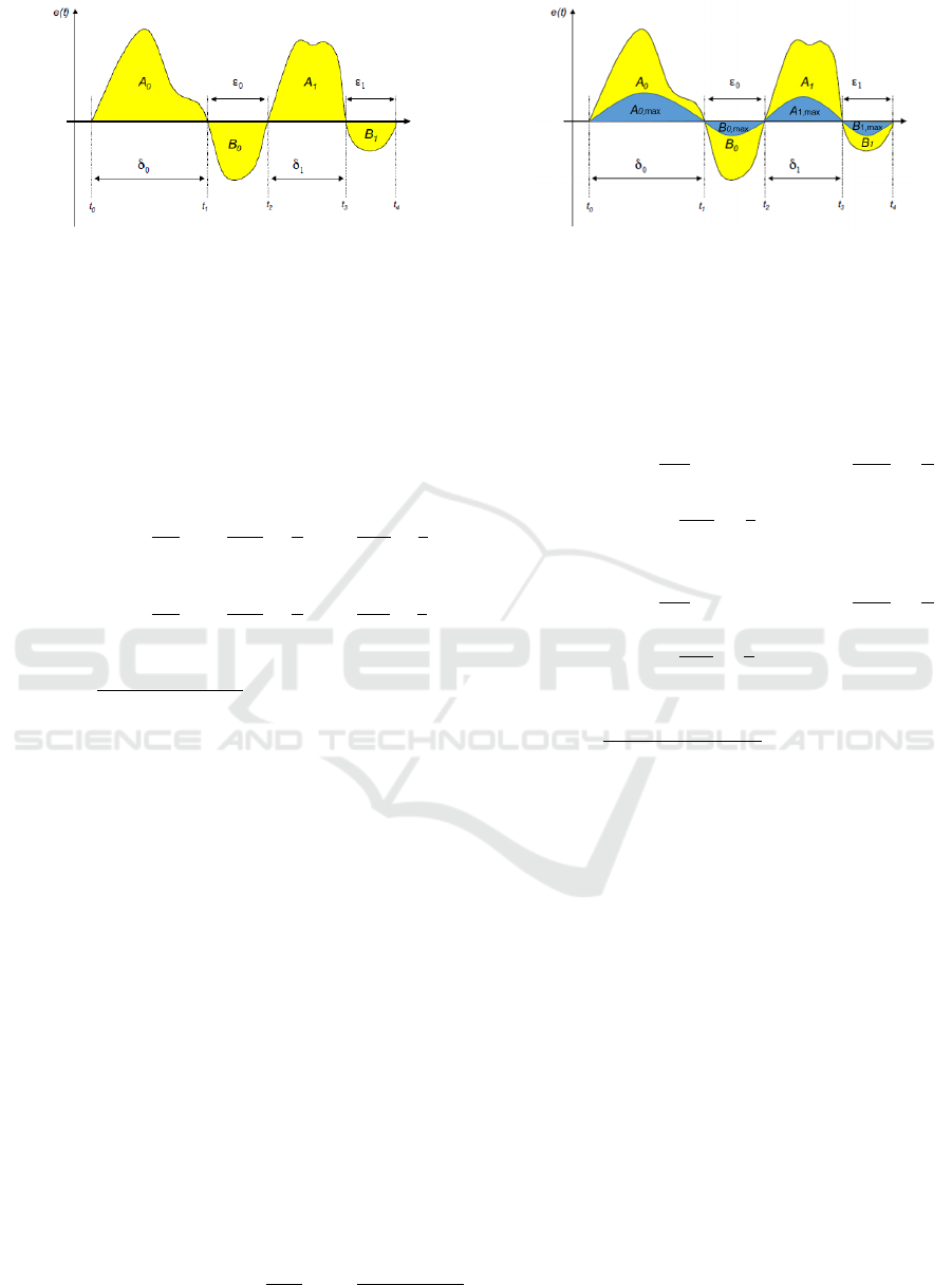
Figure 1: The Oscillation Detection Method from (Forsman

and Stattin, 1999).

ity between every two successive zero-crossing IAEs

of the error signal. However, This method handled the

positive error IAEs and the negative error IAEs sepa-

rately. Accordingly, the similarity was examined be-

tween every tow successive areas which had the same

sign (positive or negative). This separation enabled

the deﬁned criterion to detect asymmetric oscillations.

The proposed index was deﬁned as follows:

) = #



i <

;α <

i+1

∧ γ <

i+1



(2)

) = #



i <

;α <

i+1

∧ γ <

i+1



(3)

h(N

) =

) + h

)

(4)

where #S denotes the number of elements in the

set S. A

is the IAE of the positive area i of the error

signal, B

is the IAE of the negative area i of the error

signal. δ

and ε

are the time durations of the posi-

tive and the negative areas i respectively. N

is the

number of the considered successive zero-crossings.

0 < α < 1 and 0 < γ < 1 are tuning parameters deﬁne

the degree of similarity. It was suggested in (Fors-

man and Stattin, 1999) to chose α = 0.5 − 0.7 and

γ = 0.7 − 0.8.

In this work, the two previously mentioned in-

dexes will be combined. i. e. both the similarity and

the maximum area of the zero-crossing regions will

be considered to detect oscillation.

This is done simply by adding another condition to the

calculation of the index h of the second method where

the values of h

and h

increases only if A and B are

bigger than maximum limits A

max

and B

max

respec-

tively. This modiﬁcation on the second method will

increase its robustness against low amplitude noises,

which might be detected as potential oscillations. The

maximum limits are deﬁned as follows:

max

∆t

0.01e

max

sin(

πt

∆t

)dt =

0.02∆t

max

(5)

Figure 2: The Proposed Oscillation Detection Method.

With ∆t

being the time between the two corre-

sponding zero-crossings and e

max

is the previously de-

ﬁned limit of the position error.

Based on the foregoing, the modiﬁed index for os-

cillations detection becomes:

) =#

i <

< A

i,max

∧ α <

i+1

∧ γ <

i+1

(6)

) =#

i <

< B

i,max

∧ α <

i+1

∧ γ <

i+1

(7)

h(N

) =

) + h

)

(8)

Because the used controller here is only a PD con-

troller and no integral gain is applied, it is not guaran-

teed that the error signal will oscillate around the zero

value. Therefore, instead of using the error signal, it

is chosen to use the difference between the error sig-

nal and its mean value e(t) − mean(e(t)), which will

rescale the oscillating signal around the zero value.

Finally, the proposed procedure to detect oscillations

is achieved by the following steps:

1. After the beginning of the robot movement, record

the values of the position error through a long

enough period ∆T . A reasonable value of ∆T is

0.1T

tot

− 0.2T

tot

, where T

tot

is the total duration

of the robot movement.

2. Calculate the function e

(t) = e(t) − mean(e(t))

along the period ∆T .

3. Determine and count the zero-crossing points, and

calculate the values A, B, δ, ε between these

points.

4. For every N

successive zero-crossings, calculate

, h

and h.

ICINCO 2017 - 14th International Conference on Informatics in Control, Automation and Robotics

5. If h > h

max

, oscillations exist and the movement

must be stopped immediately. Otherwise, record

the values of the position error for the next period

∆T and repeat the previous steps until reaching

the end position of the robot.

It was suggested in (Forsman and Stattin, 1999) to

choose h

max

∈ [0.4 − 0.8] and N

≥ 20.

3 PARTICLE SWARM

OPTIMIZATION

After deﬁning the optimization problem and the nec-

essary constraints, It is now possible to choose one

of the optimization methods to ﬁnd the optimal gains.

The chosen method in this work is the particle swarm

optimization (PSO).

The PSO, ﬁrst introduced in (Eberhart and Kennedy,

1995), is a population-based algorithm simulating the

movement of a swarm of particles in a predeﬁned

space. After a number of iterations, the particles are

attracted towards the optimal location and gathered

around it. This location deﬁnes the optimal solution

of the problem.

The PSO has many features that make it efﬁcient in

solving optimization problems, e. g. it has less pa-

rameters to be identiﬁed in comparison with other op-

timization methods and has a very high success rate

in ﬁnding the global minimum (Rezaee Jordehi and

Jasni, 2013), and it has also a relatively high conver-

gence speed to a near optima (Angeline, 1998).

In our case, each particle position represents a vector

with a number of elements equals to the total num-

ber of gains. The main contribution of this research

is to propose a practical implementation of the PSO

method for robotic manipulators.

3.1 Deﬁning the PSO Parameters

For every iteration of the PSO algorithm, every parti-

cle of the swarm will have a new position and velocity

assigned to it based on the following equations:

(i + 1) = ω(i)V

(i) + c

(i) − X

(i))

+ c

(G(i) − X

(i))

(9)

(i + 1) = X

(i) + V

(i + 1)

(10)

Where i indicates the current iteration, j indicates

a particle of the swarm, X

(i) is the position vector

of the particle j, V

(i) is the velocity vector of the

particle j, c1 and c2 are the cognitive and the social

acceleration coefﬁcients respectively, ω(i) is the iner-

tia factor and γ

and γ

∈ [0 1] are random variables

with uniformly distributed values.

There is no standard way to choose the swarm size

and the maximum number of iterations. However,

both parameters must be high enough in order to guar-

antee a convergence of the objective value toward the

global minimum.

Regarding the inertia weight, a dynamically changing

inertia leads to better results than a constant one, and

deﬁning ω as a linear decreased function is an effec-

tive and reasonable choice as it was proven in (Shi

and Eberhart, 1999) and (Bansal et al., 2011). In this

work, the inertia weight is given as follows:

ω = ω

max

−

(ω

max

− ω

min

max

. (11)

where N

max

is the maximum number of iterations, N

is the current number of iterations, ω

max

and ω

min

are

the maximum and the minimum values of the inertia

weight respectively. The chosen values in this work

are ω

max

= 0.9 and ω

min

= 0.4 as it was suggested in

(Shi and Eberhart, 1998).

Based on the stability conditions that was introduced

in (Perez and Behdinan, 2007), it is possible to deﬁne

the parameters c1 and c2 in a way that guaranties a

convergence toward an equilibrium point eventually.

These conditions are:

0 < c1 + c2 < 4 (12)

(c1 + c2)

− 1 < ω < 1 (13)

Considering that ω ∈ [0.4 − 0.9], choosing c1 = c2 =

1 is suitable.

3.2 Constraints Handling

After deﬁning the PSO parameters, one step is only

needed before applying the method on the robot,

which is ﬁnding a suitable way to handle the con-

straints that were deﬁned in the last section. The

mostly used methods to handle constraints in PSO are

either penalty-based methods, where a penalty value

is added to the cost function if the particle position

violates any constraints, or methods that try to deﬁne

the feasible regions in the search space and restrict the

particle positions to be always inside these regions.

Unfortunately, the practical nature of the optimization

problem in this work makes both methods unsuitable.

As it was mentioned before, if one of the constraints is

violated, the movement of the robot must be stopped

immediately, which means that the cost function IAE

cannot be calculated for this movement and, there-

fore, no penalty-based method can be used. Besides,

the feasible region cannot be deﬁned theoretically in

advance and the only way to detect a violation of con-

straints is by performing the movement that results

A Practical Approach for the Auto-tuning of PD Controllers for Robotic Manipulators using Particle Swarm Optimization

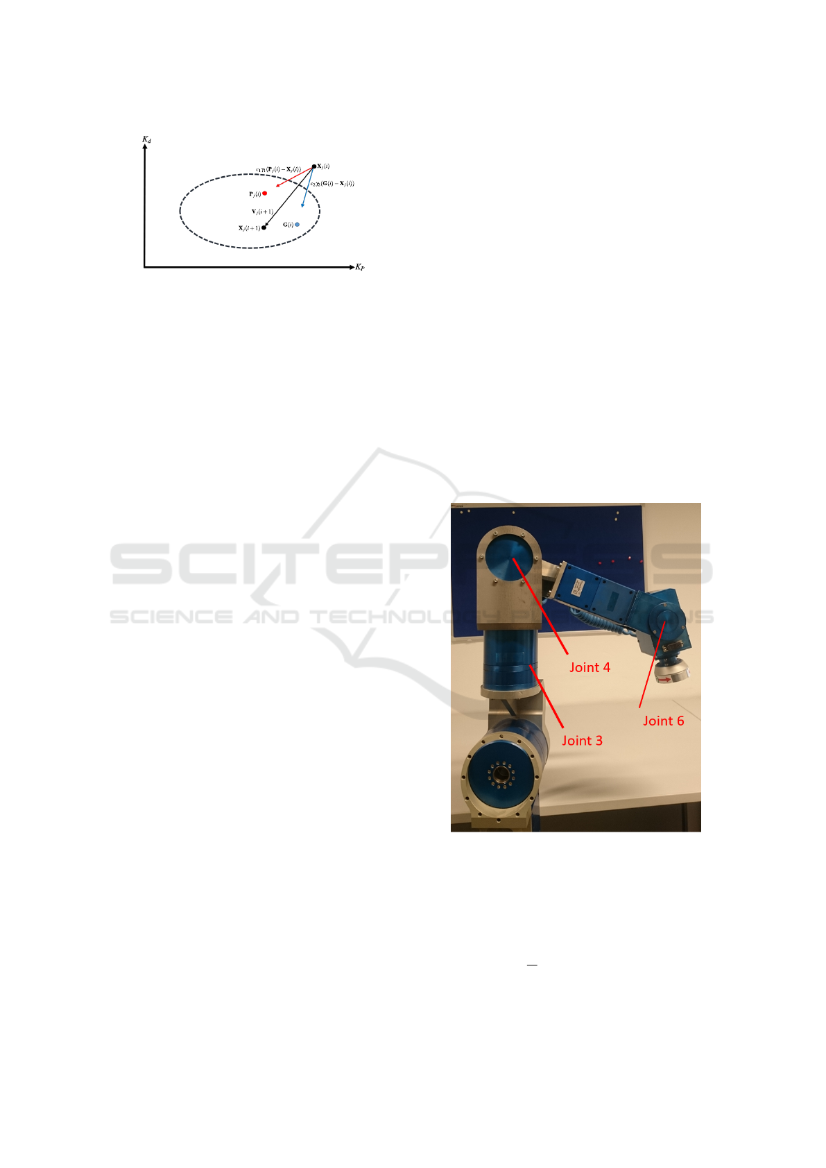
Figure 3: Constraints Handling Method.

according to the particle position.

The proposed method here to handle the con-

straints was inspired by the work in (Venter and

Sobieszczanski-Sobieski, 2003), where modiﬁcations

of the optimization method were suggested. The Han-

dling method is done after considering the following

simpliﬁcations:

• Assume that one constraint corresponding to the

link l is violated, if we ignored the coupling ef-

fects between the robot links, one can state that

the gains K

and K

of the corresponding con-

troller are only responsible for this violation and

must be modiﬁed, i. e. handling the constraints

can be done by modifying the particle position in

only two dimensions.

• There is only one continuous feasible region in-

side the search space, i. e. if a particle moves in a

direction that leads to a constraint violation, con-

tinuing to move the particle in the same direction

will also lead to a constraint violation.

• Most of the initial swarm positions are located in-

side the feasible region.

based on these simpliﬁcations, a proper method to

keep the particles inside the feasible region can be

achieved as follows:

If one of the constraints of the link l is violated, the

exploration term (ωV

) for the corresponding dimen-

sions are set to zero, which will restrict the next move-

ment in theses two dimensions to be only inﬂuenced

by the personal and the global best positions as it is

shown in ﬁgure 3. Off course these positions are lo-

cated in the feasible region, therefore, the resulted ve-

locity victor will bring the particle back to the feasible

region.

The Assumption of having only one feasible re-

gion is a reasonable assumption, because it indicates

that if a gain value violated one of the constraints after

it was increased, then continuing to increase it (while

keeping the other gains with the same values) will

keep violating this constraint. The same applies for

when the gain is decreased.

Based on the foregoing, it is now only required to lo-

cate the initial swarm inside the feasible region. A

simple strategy is to deﬁne only one suitable position

p,0

d,0

} (e. g. by tuning the controller through

trails and errors). After that, one can deﬁne an interval

in the neighborhood of this position, let it be for ex-

ample {[K

p,0

−∆K

p,0

+∆K

],[K

d,0

−∆K

d,0

∆K

]}. Finally, random initial positions can be allo-

cated with a uniﬁed distribution in this interval. It is

possible that some of the initial positions may violate

one or more of the constraints (if the chosen interval is

too large), however, they will return in the following

iterations to the feasible region thanks to the proposed

method.

4 EXPERIMENTAL RESULTS

The proposed tuning method has been tested on a 7-

DOF robot, which is built of specially designed mod-

ules called PowerCube from the company “Schunk”.

The experiment was carried on for the joints (3,4,6)

of the robot as it is shown in ﬁgure 4. All the joints

are rotational and actuated by brushless dc-motors.

Figure 4: PowerCube Robot.

The trajectory tracking performance of the PD

controllers of the robot is tested according to the de-

sired trajectories shown in ﬁgure 5. These trajectories

represent point-to-point movements with sinusoidal

velocity proﬁles.

To deﬁne the constraints for the chosen joints,

the value e

max

≈ 0.035[rad] was chosen as the

maximal position error. The PowerCube modules

provide the user with current measurements for

ICINCO 2017 - 14th International Conference on Informatics in Control, Automation and Robotics

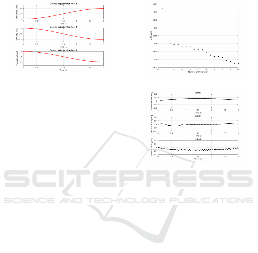
Figure 5: Desired Trajectories in Joint Space.

every motor instead of torque measurements, that

is why a maximum current constraints is used in

the experiment instead of a maximum torque. The

maximum allowed current in all of the modules

equals 15[A], but for the optimization procedure

only the half of this value is deﬁned as the current

limit (I

max

= 7.5[A]). Oscillations detection is carried

on after detecting at least N

= 20 zero-crossings

of the rescaled error signal e

(t). if the condition

h(N

) > 0.5 is met, then oscillations are considered

to be occurred and the movement of the robot must

be stopped.

Regarding the PSO algorithm, a swarm size of 10 par-

ticles is chosen and the maximum number of genera-

tions is set to 20. In addition, a tolerance value of the

cost function is set to 0.03[rad.s]. To deﬁne initial po-

sitions for the particle swarm, an acceptable gain set

of values was deﬁned through trials and errors which

are K

p,0

= [90,60,120] and K

d,0

= [5,2,8]. Based

on these values, two intervals for the initial gains are

deﬁned as follows: [K

p,0

− K

p,0

/2 K

p,0

+ K

p,0

/2]

and [K

d,0

− K

d,0

/2 K

d,0

+ K

d,0

/2].

The initial positions were then determined randomly

from inside this interval with a uniform distribution.

The search space for all the K

gains is deﬁned to

be [1 − 500] and for the K

gains [0 − 50], which

make the maximum gain limits be relatively high

compared to the initial gains. However, the maximum

velocity value V

max

was set to be equal 20% of these

maximum limits in order to avoid big leaps in the

particle movement.

After applying the PSO on the PD-controllers for the

three joints of the robot, the following optimal gain

values was found:

= {182.20, 107.46,205.8} and K

{10.29,5.55,17.83}. The optimal objective value is:

IAE = 0.0376[rad.s].

The convergence of the objective value during the

searching procedure is shown in ﬁgure 6, while ﬁgure

7 shows the position error diagram according to the

optimal gain values.

One may notice that some low amplitude oscillations

Figure 6: Convergence of the Objective Value After 20 Gen-

erations.

Figure 7: Position Error Signals According to the Optimal

Gains.

appear on the error diagram of the joint 6. These

oscillations, however, are not high enough to violate

the oscillation constraint. The fact that the optimal

gains are causing such oscillations indicates that there

is a tradeoff between the tolerated oscillations and

the accuracy of the trajectory tracking movement.

This also means that the PSO technique was able to

direct the particles toward the limits of the feasible

region to the position were the optimal gain values

are expected to be.

5 CONCLUSION

In this paper, an auto-tuning method of PD-controllers

for robotic manipulators has been proposed. The sug-

gested approach uses the particle swarm optimiza-

tion in order to ﬁnd the optimal control parameters.

The main contribution of this work was to address

the practical challenges that faces such a task and to

propose suitable solutions for it. For this sake, the

necessary constraints that guarantee a stable and safe

movement for the robot while searching for the opti-

mal gains have been deﬁned. Additionally, a suitable

way for the PSO to handle these constraints has been

suggested. Finally, the proposed approach has been

successfully experimented on a real robot.

A Practical Approach for the Auto-tuning of PD Controllers for Robotic Manipulators using Particle Swarm Optimization

REFERENCES

Angeline, P. J. (1998). Evolutionary optimization versus

particle swarm optimization: Philosophy and perfor-

mance differences. pages 601–610.

Ayala, H. V. H. and dos Santos Coelho, L. (2012). Tuning of

pid controller based on a multiobjective genetic algo-

rithm applied to a robotic manipulator. Expert Systems

with Applications, 39(10):8968–8974.

Bansal, J. C., Singh, P., Saraswat, M., Verma, A., Jadon,

S. S., and Abraham, A. (2011). Inertia weight strate-

gies in particle swarm optimization. pages 633–640.

Bekit, B., Seneviratne, L., Whidborne, J., and Althoefer, K.

(1998). Fuzzy pid tuning for robot manipulators. In

Industrial Electronics Society, 1998. IECON’98. Pro-

ceedings of the 24th Annual Conference of the IEEE,

volume 4, pages 2452–2457. IEEE.

Craig, J. J. (2005). Introduction to robotics: mechanics and

control, volume 3. Pearson Prentice Hall Upper Sad-

dle River.

Eberhart, R. and Kennedy, J. (1995). A new optimizer using

particle swarm theory. In Micro Machine and Human

Science, 1995. MHS’95., Proceedings of the Sixth In-

ternational Symposium on, pages 39–43. IEEE.

Forsman, K. and Stattin, A. (1999). A new criterion for

detecting oscillations in control loops. pages 2313–

2316.

agglund, T. (1995). A control-loop performance monitor.

Control Engineering Practice, 3(11):1543–1551.

Johnson, M. A. and Moradi, M. H. (2005). PID control.

Springer.

Kapoor, N. and Ohri, J. (2015). Improved pso tuned classi-

cal controllers (pid and smc) for robotic manipulator.

International Journal of Modern Education and Com-

puter Science, 7(1):47.

Kim, E.-J., Seki, K., Iwasaki, M., and Lee, S.-H. (2012).

Ga-based practical auto-tuning technique for indus-

trial robot controller with system identiﬁcation. IEEJ

Journal of Industry Applications, 1(1):62–69.

Kwok, D. and Sheng, F. (1994). Genetic algorithm and

simulated annealing for optimal robot arm pid con-

trol. In Evolutionary Computation, 1994. IEEE World

Congress on Computational Intelligence., Proceed-

ings of the First IEEE Conference on, pages 707–713.

IEEE.

Llama, A. M., Kelly, R., and Santiba

nez, V. (2001). A stable

motion control system for manipulators via fuzzy self-

tuning. Fuzzy Sets and Systems, 124.

Melek, W. W. and Goldenberg, A. A. (2003). Neuro-

fuzzy control of modular and reconﬁgurable robots.

IEEE/ASME transactions on mechatronics, 8(3):381–

389.

Nahapetian, N., Motlagh, M. J., and Analoui, M. (2009).

Pid gain tuning using genetic algorithms and fuzzy

logic for robot manipulator control. pages 346–350.

Ouyang, P. and Pano, V. (2015). Comparative study of de,

pso and ga for position domain pid controller tuning.

Algorithms, 8(3):697–711.

Perez, R. and Behdinan, K. (2007). Particle swarm ap-

proach for structural design optimization. Computers

& Structures, 85(19):1579–1588.

Pierezan, J., Ayala, H. H., da Cruz, L. F., Freire, R. Z., and

Coelho, L. d. S. (2014). Improved multiobjective par-

ticle swarm optimization for designing pid controllers

applied to robotic manipulator. In Computational In-

telligence in Control and Automation (CICA), 2014

IEEE Symposium on, pages 1–8. IEEE.

Rezaee Jordehi, A. and Jasni, J. (2013). Parameter selec-

tion in particle swarm optimisation: a survey. Journal

of Experimental & Theoretical Artiﬁcial Intelligence,

25(4):527–542.

Shi, Y. and Eberhart, R. C. (1998). Parameter selection in

particle swarm optimization. pages 591–600.

Shi, Y. and Eberhart, R. C. (1999). Empirical study of par-

ticle swarm optimization. 3:1945–1950.

Venter, G. and Sobieszczanski-Sobieski, J. (2003). Particle

swarm optimization. AIAA journal, 41(8):1583–1589.

ICINCO 2017 - 14th International Conference on Informatics in Control, Automation and Robotics