Design of a Sensor-based Controller Performing U-turn to Navigate

in Orchards

A. Durand-Petiteville

, E. Le Flecher

2,3

, V. Cadenat

2,3

, T. Sentenac

and S. Vougioukas

Department of Biological and Agricultural Engineering, University of California, Davis, CA, 95616, U.S.A.

CNRS, LAAS, 7 avenue du colonel Roche, F-31400 Toulouse, France

Univ. de Toulouse, UPS, LAAS, F-31400, Toulouse, France

Keywords:

Mobile Robots, Sensor-based Control, Orchard Navigation, Spiral Following.

Abstract:

In this work, the problem of designing sensor-based controllers allowing to navigate in orchards is considered.

The navigation techniques classically used in the literature rely on path following using metric maps and met-

ric localization obtained from onboard sensors. However, it appears promising to use sensor-based approaches

together with topological maps for two main reasons: ﬁrst, the environment nature is rather changing and

second, only high-level information are sufﬁcient to describe it. One of the key maneuver when navigating

through an orchard is the u-turn which must be performed at the end of each row to reach the next one. This

maneuver is generally performed using only dead reckoning because of the lack of dedicated sensory data. In

this paper, we propose two sensor-based control laws allowing to perform u-turns, improving the performance

quality. They allow following particular spirals which are deﬁned from laser rangeﬁnder data and adapted to

realize the desired maneuver. Their stability is studied and their performances are thoroughly examined. Fi-

nally, they are embedded in a complete navigation strategy to show their efﬁciency in our agricultural context.

1 INTRODUCTION

To meet the demands of nine billion people in 2050,

scientists predict that the agricultural production has

to double (Foley et al., 2011). Robotics has been iden-

tiﬁed as one of the solutions with the highest poten-

tial to achieve this goal (Reid, 2011). Indeed, robots

can improve the efﬁciency of each process of the

crops production: ﬁeld preparation, seeding/breeding,

transplanting, planting, growing, maintenance, har-

vesting, sorting and packing. To successfully perform

most of those tasks, the navigation is one of the key

challenges. Indeed the robot has to safely drive up

along one row, turn at the end of the row and enter the

next one (Siciliano and Khatib, 2016). For open ﬁeld

crops, e.g. wheat or lettuce, the navigation strategies

mostly rely on path following using GPS-based lo-

calization, such as the works presented in (Bak and

Jakobsen, 2004), (Fang et al., 2006), (Eaton et al.,

2009) and (Johnson et al., 2009). However, these

approaches are no more suitable for orchards crops,

e.g. apples or pears, because of poor satellite recep-

tion under thick canopies. It is then required to local-

ize and/or control robots thanks to embedded sensors

such as inertial units, cameras, lidars, radars, etc. The

work presented in (Barawid et al., 2007) focused

solely on straight line recognition of the tree rows us-

ing a laser scanner as a navigation sensor. A Hough

transform is applied to the points cloud to recognize

the tree row, which is then used to autonomously drive

the robot in the orchard. In (Hansen et al., 2011), a

metric localization is performed thanks to a 2D laser

scanner, an odometer and a gyroscope. The collected

data are then processed in three derivative free ﬁlters

in order to localize the robot. In (Zhang et al., 2014),

a mapping method takes as input readings from the

lidar and encoders as the vehicle is manually driven

around the orchard for at least two full rounds. Then,

the collected data are processed off-line to generate a

metric map, which is then permanently stored on the

vehicles on-board computer in order to navigate. In

(Bayar et al., 2015), the navigation is performed by

following metric paths. To do so, the localization and

control are based on a laser range-ﬁnder and wheels

and steering encoders. All the mentioned approaches

rely on a path following using a metric localization.

This latter has to deal with slopped and slippery ter-

rains, branches sticking out of the canopy, tall grass,

and missing trees. Moreover, the u-turns are usually

partially performed using dead-reckoning because of

172

Durand-Petiteville, A., Flecher, E., Cadenat, V., Sentenac, T. and Vougioukas, S.

Design of a Sensor-based Controller Performing U-turn to Navigate in Orchards.

DOI: 10.5220/0006478601720181

In Proceedings of the 14th International Conference on Informatics in Control, Automation and Robotics (ICINCO 2017) - Volume 2, pages 172-181

ISBN: Not Available

the absence of trees in the ﬁeld of view of the sensors

while following outside-the-row trajectories.

To overcome these limitations, we propose, based

on the work presented in (Durand-Petiteville et al.,

2015), to design an approach relying on non-metric

maps and sensor-based controllers in order to navi-

gate in an orchard. First, having an up to date met-

ric map of the orchards seems challenging because of

the changing nature of the environment. Indeed, over

the years, the trees grow and are pruned; over the sea-

sons, the leaves grow and disappear; over the days, the

fruits grow, bend the branches and ﬁnally fall. More-

over, to identify when the robot has to drive through

the row or switch from one row to the next one, only

high level localization data are required. Topologi-

cal maps being barely sensitive to local environment

modiﬁcations (i.e. size of the trees, presence or not

of leaves, position of the branches, ...) and providing

high level localization, they seem relevant to model

the orchard. Then, when navigating in an orchard, the

robot main goal is not to reach a destination, but to

locally behave appropriately. Indeed, it has to drive

through a row while staying at a deﬁned distance with

respect to the trees when picking fruits, or to follow a

local path when switching from one row to the other.

For this reason, it looks appropriate to use sensor-

based controllers

In this paper, we focus on the sensor-based controllers

required to navigate in an orchard. First, driving

through the row consists in following the line in the

middle of the trees. It exists a large collection of

controllers performing such a task, e.g. simple PID

controllers. To complete the navigation system, the

challenge consists in designing a sensor-based con-

troller allowing to perform a u-turn to switch from

one row to the next one. In this paper, we propose

to address this issue by designing two sensor-based

controllers following spirals around a point of inter-

est. The ﬁrst one allows to follow a spiral whose dis-

tance to the center is not known whereas the second

one follows a spiral at a known distance from it. The

design of the controllers relies on the work presented

in (Boyadzhiev, 1999) which describes how insects

ﬂy around a point of interest by performing a spiral.

In other words, it shows how to follow a path, a spi-

ral in this particular case, by simply knowing the co-

ordinates of a point of interest in the moving object

frame. This work has already been used on a UAV

(Mcfadyen et al., 2014) and a ground robot (Futter-

lieb et al., 2014) to design sensor-based controllers

avoiding obstacles. The relative position of the obsta-

Sensor-based controllers only use the data regarding the

surrounding environment and provided by the embedded

sensors.

cle with respect to the robot is used to push the robot

away from danger. Thus, the robots modify their be-

havior without following a path/spiral. The work pre-

sented in this paper aims at designing controllers fol-

lowing spirals. Thus, by tracking a point of interest, a

tree in our case, it will become possible for the robot

to actually follow a path ending in the next row.

The work is presented as follows. In the next sec-

tion the spiral model is brieﬂy summarized. Then two

controllers allowing to perform a spiral following are

designed in section 3. Next, some simulations results

showing the efﬁciency of our approach are presented.

In a last section, an example of sensor-based naviga-

tion architecture is ﬁrst presented, then simulations of

a navigation in an orchard are provided.

2 SPIRAL

Spirals have been studied in (Boyadzhiev, 1999),

where the author presents a large variety of equations

to model them. The present work focuses on some

ideas extracted from (Boyadzhiev, 1999) and more es-

pecially on the one claiming that a spiral can be seen

as the path described by a point O

moving on a plane

with respect to a ﬁxed point O

. From now on this

point will be considered as the center of the spiral.

∗

is the velocity vector applied to O

and its norm is de-

noted v

∗

(t). Moreover

∗

is the vector connecting O

to O

whose norm is d

∗

(t). Finally α

∗

(t) is deﬁned as

the oriented angle between

∗

and

∗

−→

∗

−→

∗

−→

∗

−→

∗

−→

∗

−→

∗

−→

∗

−→

∗

Figure 1: Spiral model.

In (Boyadzhiev, 1999) it is shown that if both v

∗

(t)

and α

∗

(t) are constant then O

describes a spiral

whose center is O

. For this reason they are respec-

tively denoted v

∗

and α

∗

from now on. Moreover

the author provides an important equation regarding

∗

(t):

∗

(t) = −v

∗

cos(α

∗

) (1)

As it can be seen in this equation, the type of spiral

performed depends on the sole parameter α

∗

. First

if 0 < α

∗

< π, O

turns counter-clockwise with re-

Design of a Sensor-based Controller Performing U-turn to Navigate in Orchards

173

-5 0 5

X(m)

-4

-2

Y(m)

(a) Inward spiral - α

∗

15π

-5 0 5

X(m)

-6

-4

-2

Y(m)

(b) Outward spiral - α

∗

17π

Figure 2: Example of spirals - Black cross: center of the

spiral - Green cross: initial position - Red cross: ﬁnal posi-

tion.

spect to O

otherwise if −π < α

∗

< 0 it turns clock-

wise. Then if 0 ≤ α

∗

< π/2 or −π/2 ≤ α

∗

< 0,

∗

(t) decreases with time (see ﬁgure 2(a)). In other

words, O

is describing an inward spiral around O

If π/2 < α

∗

≤ π or −π ≤ α

∗

< −π/2 then d

∗

(t) in-

creases with time (see ﬁgure 2(b)) which means O

is describing an outward spiral around O

. Finally,

if α

∗

= π/2 or α

∗

= −π/2, d

∗

(t) = d

∗

(0). O

then

describes a circle of radius d

∗

(0) around O

Equation (1) and its analysis highlight our interest in

spirals. Indeed, by adapting the spiral model to a

robot and then making converging α, angle between

its linear velocity vector and the point of interest O

towards α

∗

, it is possible to make the vehicle follow a

spiral deﬁned by α

∗

. Thus the sensor space is used to

control the robot path.

3 CONTROLLER DESIGN

In the previous section, it has been explained how to

choose a value for α

∗

in order to deﬁne a spiral. In

this section, controllers allowing a robot to perform

such a spiral are presented. To do so, we ﬁrst present

the model of the robot and how to adapt the spiral

approach to it. Then a ﬁrst controller following a spi-

ral only deﬁned by its α

value is designed and its

performance is analyzed. Finally a more advanced

controller allowing to follow a speciﬁc spiral, i.e. de-

ﬁned by its α

∗

value and the initial distance to O

, is

introduced.

3.1 Robot Modeling

In this work we consider the differential robot pre-

sented in ﬁgure 3. Let F

= (O

,~x

,~y

,~z

) and

= (O

,~x

,~y

,~z

) the frames respectively attached to

the world and the robot. The robot state vector is de-

ﬁned as χ(t) = [x(t),y(t),θ(t)]

, where x(t) and y(t)

are the coordinates of O

in F

, whereas θ(t) is the an-

gle between ~x

and ~x

. Finally the robot is controlled

using the input vector

χ(t) = [v(t), ω(t)]

where v(t)

is the linear velocity along ~x

, and ω(t) the angular

velocity around~z

α(t)

−→

β(t)

θ( t)

x(t)

y(t)

Figure 3: Robot model.

As previously mentioned, this work focuses on fol-

lowing a spiral whose center is denoted O

. It then

requires to adapt the spiral model to the robot. The

vector connecting O

to O

is named

d and α(t) is the

angle between ~x

and

d. It should be noticed that:

α(t) = π − θ(t) + β(t) (2)

α(t) = −

θ(t) +

β(t) = −ω(t) +

v(t)

d(t)

sin(α(t)) (3)

Finally d(t) represents the distance between O

and O

, and it can be shown (see (Boyadzhiev, 1999))

that:

d(t) = −v(t) cos(α(t)) (4)

3.2 First Approach

A ﬁrst solution to follow a spiral consists in designing

a controller which makes α(t) converge to a desired

angle named α

= α

∗

. α

determines if the spiral is

an inward one, an outward one or a circle. Once the

robot has converged towards the spiral, it either in-

creases, decreases or keeps constant d(t). In order to

design such a controller, we impose a constant linear

velocity such as v(t) = v

∗

. Then we deﬁne an error

(t) and compute ˙e

(t):

(t) = α(t) − α

(5)

˙e

(t) =

α(t) = −ω(t) +

d(t)

sin(α(t)) (6)

As it can be seen in (6), ˙e

(t) depends on both v and

ω(t). As it has been decided to ﬁx a constant linear

velocity, it is then required to compensate its effect

while controlling the robot using solely ω(t). More-

over, to make the error e

(t) vanish, we propose to

deﬁne a controller proportional to it. Thus it follows

that:

ICINCO 2017 - 14th International Conference on Informatics in Control, Automation and Robotics

174

ω(t) = λ

(t) +

v(t)

d(t)

sin(α(t)) (7)

where λ

is a positive scalar. The controller obtained

in equation (7) can be used to force the robot to follow

a spiral deﬁned by α

. Thus it is possible to control

if the robot increases, decreases or keeps constant the

distance d(t). However it does not allow to follow a

speciﬁc spiral. In order to analyze the stability of the

designed controller, we propose to deﬁne the follow-

ing Lyapunov function:

(t)) =

(t)

(8)

with x

(t) = e

(t). The equilibrium state x

(t) = 0 corresponds to the robot following the spiral

deﬁned by α

. Moreover V

(t)) > 0 for x

(t) 6=

and V

(t)) = 0 when x

(t) = x

. To study

the evolution of V

(t)), its derivative with respect

to time is computed:

(t)) = ˙x

(t)x

(t)

α(t)[α(t) − α

]

= [−ω(t) +

d(t)

sin(α(t))][α(t) − α

]

= −λ

(t)

(9)

Thanks to equation (9), it can be seen that

(t)) <

0 for x

(t) 6= x

and

(t)) = 0 when x

(t) = x

as λ

> 0. Thus we can conclude that the designed

controller has a global exponential stability.

3.3 Second Approach

The controller in equation (7) allows to control the

robot behavior, i.e. to increase, decrease or keep con-

stant the distance d(t). Nevertheless it does not allow

to follow a speciﬁc spiral. Indeed it exists an inﬁn-

ity of spirals deﬁned by α

and in order to deﬁne a

speciﬁc spiral it is mandatory to select both the an-

gle α

and the initial distance d

∗

(0). When using the

controller in equation (7), d

∗

(0) is not chosen and it

corresponds to d(t

), where t

is the time when α(t)

has converged to α

. Thus, in order to follow a spe-

ciﬁc spiral, we once again impose a constant linear

velocity such as v(t) = v

∗

. Then we propose to deﬁne

the following error:

(t) = α(t) − α

− α

ε(t) (10)

In order to make the new error e

(t) vanish, the

constant reference α

has been replaced by a non-

constant one, α

(t) = α

+ α

ε(t). The vanishing

error in equation (10) should lead to two successive

robot behaviors. First while d

∗

(t) 6= d(t), the robot

has to navigate towards the spiral in order to make

∗

(t) = d(t). To do so the new angle of reference

(t) is equal to α

modiﬁed by the amount α

∗ε(t).

is the maximal value that can be added/subtracted

to α

in order to make the robot converge towards the

spiral without changing its sense of rotation with re-

spect to the center of the spiral (clockwise or counter-

clockwise). Then ε(t) should have its norm equal to

1 when ||d(t) − d

∗

(t)|| ≥ ||d(0) − d

∗

(0)||, and equal

to 0 when d(t) = d

∗

(t). Thus, when the robot is

far from the spiral, it converges towards it using the

greater angle possible, i.e. α

(t) = 0 or α

(t) = ±π

depending on the initial conditions. Moreover, when

d(t) = d

∗

(t), then α

(t) = α

. Thus the robot follows

the spiral while keeping the desired distance. This

last part corresponds to the second behavior expected

when controlling the robot by vanishing e

(t). In or-

der to obtain the previously explained behaviors, we

propose to deﬁne ε(t) and α

as:

ε(t) = sign(d

∗

(t) − d(t)) min



∗

(t) − d(t)

∗

(0) − d(0)|

||,1



(11)

and



sign(α

) ∗ π − α

if d

∗

(0) > d(0)

if d

∗

(0) < d(0)

(12)

ε(t) is the normalized error between d

∗

(t) and d(t).

It has been saturated to ±1. Thus its value belongs

to the domain [0, 1] if d

∗

(0) > d(0) or [−1,0] if

∗

(0) < d(0). Thus, α

6= α

when d

∗

(t) 6= d(t),

whereas α

= α

when d

∗

(t) = d(t). Regarding

equation (12), when α

∈ [0,π] then it is mandatory

that α

∈ [0, π]. Otherwise when α

∈ [0, −π] then

∈ [0,−π]. Equations (11) and (12) guarantee that

the robot rotation direction is not modiﬁed by α

ε(t),

while allowing the robot to converge towards d

∗

(t).

Now that the new error has been deﬁned, we propose

to compute its derivative with respect to time in order

to identify the terms involved in its dynamics.

˙e

(t) =

α(t) − α

ε(t)

= −ω(t) +

v(t)

d(t)

sin(α(t)) − α

ε(t)

(13)

In order to make e

(t) vanish, we propose to design

a controller proportional to it which also compensate

the other terms involved in (13). It leads to:

ω(t) = λ

(t) +

v(t)

d(t)

sin(α(t)) − α

∗

ε(t) (14)

where λ

is a positive scalar. The controller (14)

makes possible for the robot to converge towards any

speciﬁc spiral. In order to analyze the stability of

the controller, we propose to deﬁne the following

Lyaponuv function:

(t)) =

(t)

+ x

(t)

(15)

Design of a Sensor-based Controller Performing U-turn to Navigate in Orchards

175

with

(t) =



(t)





α(t) − α

− α

∗ ε(t)

d(t) − d

∗

(t)



The equilibrium state x

= [x

(t),x

(t)]

= [0,0]

corresponds to the robot following the spiral deﬁned

by α

while being at the distance d

∗

(t), i.e. when

α(t) = α

and d(t) = d

∗

(t). Moreover, V

(t)) > 0

for x

(t) 6= x

and V

(t)) = 0 when x

(t) = x

. In

order to study the evolution of V

(t)), its derivative

with respect to time is computed:

(t))

= ˙x

(t)x

(t) + ˙x

(t)x

(t)

= −λ

(t)

+ [

d(t) −

∗

(t)][d(t) − d

∗

(t)]

= −λ

(t)

−v[cos(α(t)) − cos(α

)][d(t) − d

∗

(t)]

(16)

In equation (16), it can be seen that

(t)) = 0

for x

(t) = x

. However, it can not be proved

that

(t)) < 0 for x

(t) 6= x

. Indeed even

if −λ

(t)

< 0 for x

(t) 6= x

, the second term

v[cos(α(t)) − cos(α

)][d(t) − d

∗

(t)] is not always

positive. For certain initial conﬁgurations the sign

of cos(α(t)) − cos(α

) is different from the one of

d(t) − d

∗

(t). Moreover, the initial robot orientation

may not allow it to reduce ||d(t) − d

∗

(t)|| when it

starts to move. This is due to the fact that only one

control input, ω(t), is used to control the two de-

grees of freedom α(t) and d(t) of a non-holonomic

robot. Thus it might be ﬁrst required to orientate

the robot. During this orientation step the distance

||d(t) − d

∗

(t)|| increases. Thus we can conclude that

the controller is not globally asymptotically stable.

However it is straightforward to show that:

If d(t) > d

∗

(t):

cos(α(t)) − cos(α

) > 0 if α(t) > α

If d(t) < d

∗

(t):

cos(α(t)) − cos(α

) < 0 if α(t) < α

(17)

As it can be seen in equation (17), it is guaranteed that

the controller is locally asymptotically stable once the

α(t) overpasses α

. Thus the obtained results do not

completely fulﬁll our expectations, but are sufﬁcient

for our needs. A more accurate value of α(t) allowing

a local stability could be found. It would depend on

v(t), λ

and the initial conditions. Finally, as it will

be shown in the simulation section, it is possible to

sequence these two controllers to bring the robot in an

initial state where the stability of the second control

law is guaranteed.

In this section two controllers have been designed.

The ﬁrst one allows to follow a spiral having an un-

known distance d

∗

(t). It can be used when control-

ling the robot behavior, i.e. increasing, decreasing

or keeping constant d(t) This controller is sufﬁcient

when the distance is not available, eg. when the data

are provided by a single camera. The second con-

troller allows to follow a spiral while controlling d(t).

It is then required to provide d(t), using for example

a stereo camera, a Lidar, etc.

3.4 Validation

In this section we present simulations of a robot fol-

lowing a spiral using the two previously designed

controllers. The results aim to illustrate the efﬁciency

of our approach and also highlight its performances

and limitations. Moreover we will propose ideas to

investigate in order to overcome some issues and/or

adapt the presented approach to another application.

For all the simulations the sampling time is T

= 0.1

second. Moreover the coordinates of the spiral cen-

ter are [0, 0] and the linear velocity is v

∗

= v(t) = 0.2

m/s. The ﬁrst set of simulations, the results of which

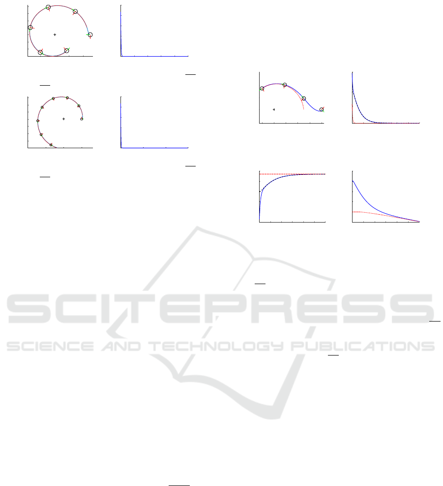
can be seen in ﬁgure 4, are performed using the ﬁrst

controller from equation (7) and λ

= 1. The ﬁrst test

aims to follow an inward spiral by using α

15π

when the robot initial state is χ(0) = [5,0,π]

(see

ﬁgure 4(a)). The second one follows an outward spi-

ral with α

17π

and an initial state χ(0) = [5, 0, 0]

(see ﬁgure 4(c)). In both ﬁgures 4(a) and 4(c), the dot-

ted red line is the path of reference whereas the solid

blue one is the path performed by the robot while us-

ing the controller from equation (7). Moreover, some

robot states, and especially the ﬁrst one, are repre-

sented. The green and red lines represent ~x

(t) and

(t), respectively. In both cases, the robot ﬁrst ori-

entates itself in order to make α(t) converge towards

, then it follows a spiral by keeping α(t) = α

. This

behavior is shown in ﬁgures 4(b) and 4(d) where the

evolution of the Lyapunov function V

(t)) is pre-

sented. Indeed x

(t)

= (α(t) − α

)

ﬁrst decreases

down to zero, and then stays at the constant null value.

This result matches with the proposed analysis pre-

sented in section 3.2. However it should be noticed

that the robot does not follow a predeﬁned spiral, but

the one met once V

(t) = 0. Thus we can conclude

that the controller from equation (7) can be used in or-

der to control the behavior of a robot with respect to

a point, i.e. it increases, decreases or keeps constant

d(t), but it does not allow to follow a speciﬁc spiral,

i.e. control the distance d(t).

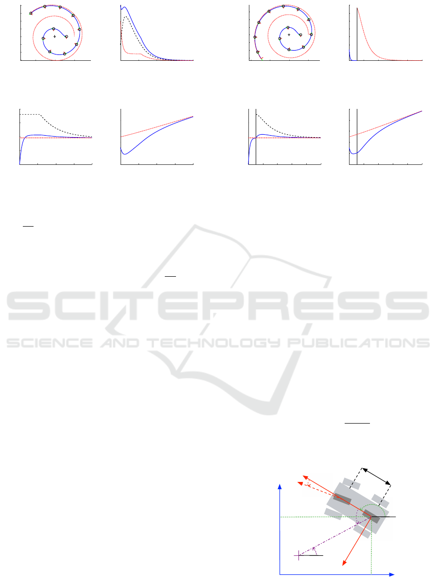
The second set of simulations uses the spiral follow-

ing controller presented in equation (14). For the ﬁrst

test (see ﬁgure 5), λ

= 1, α

15π

and d

∗

(0) = 5 m.

Moreover the robot initial state is χ(0) = [8,0,−

]

In this simulation the robot has to follow the speciﬁc

spiral deﬁned by α

15π

and passing by the point

ICINCO 2017 - 14th International Conference on Informatics in Control, Automation and Robotics

176

-2 0 2 4

X(m)

-3

-2

-1

Y(m)

(a) Robot trajectory

| α

15π

0 20 40 60 80 100

Time(s)

0.5

1.5

2.5

(t))

(b) V

(t)) | α

15π

-5 0 5

X(m)

-8

-6

-4

-2

Y(m)

| α

17π

0 50 100 150

Time(s)

0.5

1.5

2.5

(t))

(d) V

(t)) | α

17π

Figure 4: Spiral following using the ﬁrst controller - Black

cross: center of the spiral - Solid line: robot trajectory -

Doted line: spiral of reference.

whose coordinates are [5,0]. In ﬁgure 5(a), it can be

seen that the robot successfully manages to follow

the predeﬁned spiral by simultaneously orienting it-

self toward the spiral (see ﬁgure 5(c)) and making the

distance d(t) converge towards d

∗

(t) (see ﬁgure 5(d)).

Figure 5(b) presents the evolution of V

(t)), x

(t)

and x

(t). It can be seen that x

(t) = e

(t) is perma-

nently decreasing and converges towards zero. Then

it should be noticed that x

(t) = d(t) − d

∗

(t) slightly

increases before decreasing down to zero. Moreover

it vanishes after x

(t). This behavior is due to the fact

that the non-holonomic robot is initially not well ori-

ented. Thus, while orienting itself, x

(t) increases.

Once the robot is correctly oriented towards the spiral,

vanishing e

(t) allows the robot to converge towards

the speciﬁc spiral and then to follow it. It can be

also seen that V

(t)) is constantly decreasing and

is then equal to zero when the robot is on the spiral.

In this test the increase of x

(t) due to the orientation

step is not large enough with respect to the reduction

of x

(t) to not allow V

(t)) to be constantly de-

creasing. Those results match the stability analysis

proposed in section 3.3. First, V

(t)) =

(t)

can-

not be used as a Lyapunov function to guarantee that

the robot follow a spiral. Indeed, x

(t) = 0 before the

robot is on the spiral. Then, only an appropriate ori-

entation of the robot guarantees the decrease of x

(t)

and then V

(t)). However, despite of not being ini-

tially well oriented, the robot manages to perform its

task successfully. Finally it should be noticed that in

our case, the robot is always moving forward. A so-

lution to obtain an monotonically decreasing x

(t)

could be to allow the robot to move backward in or-

der to perform a maneuver. This solution has not been

selected in this work because the designed controllers

have to be used to perform obstacles avoidance or u-

turn while navigating. Moving backward would be an

inappropriate motion with respect to such a naviga-

tion task.

-2 0 2 4 6 8

X(m)

-2

Y(m)

(a) Solid line: Robot tra-

jectory - Dotted line: ref-

erence spiral

0 10 20 30 40 50 60

Time(s)

(t)) | x

(t) | x

(t)

(b) Solid line: V

- Dot-

ted line: x

- Dashed line:

0 10 20 30 40 50 60

Time(s)

-150

-100

-50

100

α(t) vs α

(deg)

ted line: α

- Dashed line:

(t)

0 10 20 30 40 50 60

Time(s)

d(t) vs d

(t) (m)

(d) Solid line: d(t) - Dot-

ted line: d

∗

(t)

Figure 5: Spiral following using the second controller with

15π

For the second simulation using the controller given

by equation (14) (see ﬁgure 6), λ

= 0.2, α

17π

and d

∗

(0) = 5 m. Moreover, the robot initial state is

χ(0) = [3,0,π]. The robot has to follow the speciﬁc

spiral deﬁned by α

17π

and passing by the point

whose coordinates are [5,0]. As previously the robot

successfully follows the predeﬁned spiral even if the

time to converge towards it is much greater than be-

fore (see ﬁgure 6(a)). Similarly to the previous sim-

ulation the initial robot state requires an orientation

step leading to an increase of x

(t) (see ﬁgures 6(d)

and 6(b)). Moreover, in order to make x

(t) vanish,

α(t) has to overshoot α

(see ﬁgure 6(c)). This is due

to the term α

∗ε(t) in equation (10). However it does

not lead to any increase of x

(t) over the spiral fol-

lowing (see ﬁgure 6(b)). In this particular simulation,

having λ

= 0.2 introduces an increase of V

(t))

at the beginning of the simulation. Indeed, the varia-

tions of x

(t) due to the orientation step are no more

compensated by the strong decrease of x

(t). One

more time the reduction of V

(t)) is only guaran-

teed once the robot is correctly oriented with respect

to the spiral. Despite this issue in term of stability

analysis, the robot manages to converge towards the

spiral and then to follow it.

In a last simulation (see ﬁgure 7), we propose to use

successively both controllers. The spiral to follow, the

robot initial state and the parameter values are identi-

Design of a Sensor-based Controller Performing U-turn to Navigate in Orchards

177

-5 0 5

X(m)

-6

-4

-2

Y(m)

(a) Solid line: Robot trajec-

tory - Dotted line: reference

spiral

0 50 100 150 200

Time(s)

(t)) | x

(t) | x

(t)

(b) Solid line: V

- Dotted

line: x

- Dashed line: x

0 50 100 150 200

Time(s)

100

150

200

α(t) vs α

(deg)

ted line: α

- Dashed line:

(t)

0 50 100 150 200

Time(s)

d(t) vs d

(t) (m)

(d) Solid line: d(t) - Dotted

line: d

∗

(t)

Figure 6: Spiral following using the second controller with

17π

cal to the previous simulation. Initially the robot is

controlled using the ﬁrst controller and thus it fol-

lows a non-speciﬁc spiral having α

17π

. Once

α(t) = α

, the robot then switches to the second con-

troller to follow the spiral having α(t) = α

and pass-

ing by the point with coordinates [5, 0]. This approach

allows to obtain the robot to reach an initial state

that guarantees the convergence of the second con-

troller. Indeed, in ﬁgure 7(b), it can be seen that both

(t)) and V

(t)) are decreasing. Other than

the Lyapunov functions, the path and the evolution of

α(t) and d(t) are almost the same as in the previous

simulation (ﬁgures 7(a) 7(c) and 7(d)). This approach

allows to guarantee the convergence of the robot to-

wards a speciﬁc spiral despite its initial state, but it

does not drastically change its performances.

4 NAVIGATION STRATEGY

In this section we propose to present how the sensor-

based spiral controller can be used into a navigation

architecture to allow a robot to drive through an or-

chard. First, a possible navigation is described: robot,

sensors, map, controllers and supervision. Then, we

present results obtained in simulation to highlight the

efﬁciency of the sensor-based approach.

-10 -5 0 5

X(m)

-6

-4

-2

Y(m)

(a) Solid line: Robot trajec-

tory - Dotted line: reference

spiral

0 50 100 150 200 250

Time(s)

(t))

(b) Solid line: V

- Dotted

line: V

0 50 100 150 200 250

Time(s)

100

150

200

α(t) vs α

(deg)

ted line: α

- Dashed line:

(t)

0 50 100 150 200 250

Time(s)

d(t) vs d

(t) (m)

(d) Solid line: d(t) - Dotted

line: d

∗

(t)

Figure 7: Spiral following using successively both con-

trollers. The switch occurs at t = 26.2 s.

4.1 Robot and Sensory Data

To navigate through the orchard, we consider the

Toro workman MDE vehicle, which is a car-like

robot equipped with three laser rangeﬁnders (see

ﬁgures 8 and 9). The state vector is χ

(t) =

[x(t),y(t), θ(t), γ(t)]

, with γ(t) the steering angle,

and the input vector is u

(t) = [v(t),γ(t)]

. It should

be noticed that the second term of the control input

vector, which used to be an angular velocity for the

differential model, is now an angular position. It is

then required to convert the angular velocity ω(t) to

an angular position γ(t) allowing the robot to rotate

by the same amount. To do so, we use the following

equation:

γ(t) = tan

−1

(

L ω(t)

v(t)

) (18)

where L is the distance between the front axle and the

rear axle.

α(t)

−→

β(t)

θ( t)

x(t)

y(t)

γ(t)

Figure 8: Car-like model.

ICINCO 2017 - 14th International Conference on Informatics in Control, Automation and Robotics

178

The ﬁrst laser rangeﬁnder mounted in front of the

robot and facing towards, aims at detecting the trees

in order to drive trough the rows. The acquired data

are processed in order to identify the trees in the ﬁeld

of view of the laser rangeﬁnder (the circled trees in

ﬁgure 9). Next the trees are separate into two clus-

ters: left row (red circles) and right row (green cir-

cles). Next, the best ﬁtting lines ∆

and ∆

are calcu-

lated for the left and right cluster respectively. Then,

∆

, the line median to ∆

and ∆

is computed. Fi-

nally, the orientation error ε

and the lateral position

error ε

are calculated in the front rangeﬁnder frame

= (O

,~x

,~y

,~z

)

(see ﬁgure 9). These last two

values are used to drive through the row.

Figure 9: Data acquisition during a row following.

Two laser rangeﬁnders are mounted at the back of the

robot and face the right and left sides respectively (see

ﬁgure 9). They are used to detect the trees when per-

forming a u-turn. The data acquired in the rangeﬁnder

frame are ﬁrst projected in the robot frame. Next,

they are processed to detect the closest tree. Then,

the angle α(t) and the distance d(t) are computed in

the robot frame (see ﬁgure 10). These values are used

to control the robot while performing a u-turn.

4.2 Environment Modeling

In this simulation, we consider an orchard composed

of 4 rows made of 8 trees (see ﬁgure 11). It forms tree

rows for the robot to navigate through.The rows width

is 8 meters whereas the trees are spaced by 3 meters.

To model the orchard, we have chosen to use the topo-

logical map presented in ﬁgure 12 which consists in

an oriented graph. Here, the nodes (U

), (U

)

and (U

) represent the ﬁrst, second and third row

respectively. U

is used when the robot drives upward

These parameters have to expressed in the robot frame.

However, their values are the same in F

and F

Figure 10: Data acquisition during a u-turn.

in row x, whereas D

is used when it drives down-

ward. The nodes R

and L

represent the right and

left turns from row y towards row z. At the begin-

ning of the navigation, the user provides initial and

ﬁnal nodes. Thanks to these informations, a path is

computed. For example from U

to U

the path is

P = {U

Figure 11: Simulated orchard.

Figure 12: Topological map.

Design of a Sensor-based Controller Performing U-turn to Navigate in Orchards

179

4.3 Control Strategy

Over the navigation, the robot is controlled using two

controllers. The ﬁrst one allows the robot to drive

through the rows while staying in the middle of it. It

is deﬁned as:

ω = λ

+ λ

(19)

where λ

and λ

are two positive scalar gains. Next,

the controller to perform a u-turn, is one of the two

ones previously presented, i.e. either controller (7) or

(14). Finally, it has to be determined when the robot

has to switch from one controller to the other based on

the data provided by the on-board sensors. First, it is

required to switch from the row following controller

to the u-turn one when i) the front laser range ﬁnder

does not perceive a tree anymore, ii) α

l,r

< |π/2 + ε

where α

l,r

are the α(t) values provided by the left and

right camera and ε

is a very small angle. In other

words, the robot has to be at the end of the row, with

the two side laser rangeﬁnders at the level of the last

two trees. Finally, the robot switches from the u-turn

mode to the row following one, when the side sensor

which is not used to perform the u-turn perceives two

trees. It should be noted that the linear velocity is

deﬁned by the user when both following the rows and

performing a u-turn.

4.4 Validation

The presented navigation strategy has been imple-

mented in ROS and coupled with Gazebo in order

to provide a simulation environment. The following

gains have been selected: λ

= 1, λ

= 5 and

= 5. Moreover the linear speed is v(t) = 2 m/s

when the robot is in the rows, whereas v(t) = 1 m/s

when it performs a u-turn. Finally α

= ±π/2, forc-

ing the robot to follow a circle when switching rows.

During the ﬁrst simulation, the robot starts at D

and

follows the path P = {D

}. In order

to switch rows, controller (7) is used. As it can be

seen in ﬁgure 13, the robot successfully switch from

one controller to the other in order to navigate through

the orchard and reach its destination. During L

and

, the distance to the trees is not controlled. How-

ever, because it is initially located at the center of the

row, the robot manages to switch rows.

In a second simulation the controller (14) is used to

switch rows. The robot starts in U

and has to fol-

low the path P = {U

}. Once again,

it manages to use both controllers to drive through the

orchard and reach the goal. In R

and L

, the dis-

tance to the trees is controlled and ﬁxed to 4 m. It

allows to guarantee that the robot will enter the n the

middle of the following row.

Figure 13: Orchard navigation #1.

Figure 14: Orchard navigation #2.

5 CONCLUSION

We have considered the problem of designing sensor-

based controllers allowing to navigate in orchards.

More particularly, we have focused on the realiza-

tion of u-turns which are traditionnally realized using

deadreckoning only. To improve the quality of the

maneuver, we have developed two sensor-based con-

trollers. They allow to follow particular spirals which

are deﬁned from laser data and adapted to realize the

desired maneuvre. It is important to note that the per-

formances are different for both controllers. The ﬁrst

one allows to follow a spiral, but the distance to its

center is not controlled. The second controller is more

advanced and allows to follow a speciﬁc given spiral,

i.e. angle α(t) and distance d(t) are controlled. In this

approach data from the sensor space are sufﬁcient to

ICINCO 2017 - 14th International Conference on Informatics in Control, Automation and Robotics

180

control the robot path. No localization are required

with the proposed method. In addition a stability anal-

ysis of those controllers and simulations highlighting

the efﬁciency of our approach have been provided. In

a second step, we have embedded them in a complete

navigation strategy allowing to navigate through an

orchard. We have explained how the different data

necessary for the control are derived, how the environ-

ment is modeled and how the robot is controlled using

the appropriate controllers. Finally a complete simu-

lation using ROS and Gazebo shows the efﬁciency of

the chosen approach in our agricultural context. The

next step of our work is to implement the controllers

on the Toro workman MDE robot. Finally, we also

plan to develop this sensor-based approach and take

advantage of its reactivity in order to navigate in a

dynamic environment.

REFERENCES

Bak, T. and Jakobsen, H. (2004). Agricultural robotic plat-

form with four wheel steering for weed detection.

Biosystems Engineering, 87(2):125–136.

Barawid, O. C., Mizushima, A., Ishii, K., and Noguchi,

N. (2007). Development of an autonomous naviga-

tion system using a two-dimensional laser scanner

in an orchard application. Biosystems Engineering,

96(2):139–149.

Bayar, G., Bergerman, M., Koku, A. B., and ilhan Konuk-

seven, E. (2015). Localization and control of an au-

tonomous orchard vehicle. Computers and Electron-

ics in Agriculture, 115:118–128.

Boyadzhiev, K. N. (1999). Spirals and conchospirals in the

ﬂight of insects. The College Mathematics Journal,

30(1):21–31.

Durand-Petiteville, A., Cadenat, V., and Ouadah, N. (2015).

A complete sensor-based system to navigate through

a cluttered environment. In Informatics in Control,

Automation and Robotics (ICINCO), 2015 12th Inter-

national Conference on, volume 2, pages 166–173.

IEEE.

Eaton, R., Katupitiya, J., Siew, K. W., and Howarth, B.

(2009). Autonomous farming: Modelling and control

of agricultural machinery in a uniﬁed framework. In-

ternational journal of intelligent systems technologies

and applications, 8(1-4):444–457.

Fang, H., Fan, R., Thuilot, B., and Martinet, P. (2006).

Trajectory tracking control of farm vehicles in pres-

ence of sliding. Robotics and Autonomous Systems,

54(10):828–839.

Foley, J. A., Ramankutty, N., Brauman, K. A., Cassidy,

E. S., Gerber, J. S., Johnston, M., Mueller, N. D.,

O’Connell, C., Ray, D. K., West, P. C., Balzer, C.,

Bennett, E. M., Carpenter, S. R., Hill, J., Monfreda,

C., Polasky, S., Rockstr

om, J., Sheehan, J., Siebert,

S., Tilman, D., and Zaks, D. P. M. (2011). Solutions

for a cultivated planet. Nature, 478:337–342.

Futterlieb, M., Cadenat, V., and Sentenac, T. (2014). A Nav-

igational Framework Combining Visual Servoing and

Spiral Obstacle Avoidance Techniques. In Interna-

tional Conference on Informatics in Control, Automa-

tion and Robotics ( ICINCO ) , pages 57–64, Vienna,

Austria. INSTICC.

Hansen, S., Bayramoglu, E., Andersen, J. C., Ravn, O., An-

dersen, N., and Poulsen, N. K. (2011). Orchard navi-

gation using derivative free kalman ﬁltering. In Amer-

ican Control Conference (ACC), 2011, pages 4679–

4684. IEEE.

Johnson, D. A., Nafﬁn, D. J., Puhalla, J. S., Sanchez, J., and

Wellington, C. K. (2009). Development and imple-

mentation of a team of robotic tractors for autonomous

peat moss harvesting. Journal of Field Robotics, 26(6-

7):549–571.

Mcfadyen, A., Durand-Petiteville, A., and Mejias, L.

(2014). Decision strategies for automated visual col-

lision avoidance. In Unmanned Aircraft Systems

(ICUAS), 2014 International Conference on, pages

715–725.

Reid, J. (2011). The impact of mechanization on agricul-

ture. Nat. Acad. Eng. Bridge, Issue Agric. Inf. Tech-

nol., 41(3):22–29.

Siciliano, B. and Khatib, O. (2016). Springer handbook of

robotics. Springer.

Zhang, J., Maeta, S., Bergerman, M., and Singh, S. (2014).

Mapping orchards for autonomous navigation. In

Proc. American Society of Agricultural and Biologi-

cal Engineers Annu. Int. Meeting.

Design of a Sensor-based Controller Performing U-turn to Navigate in Orchards

181