Efficient Implementation of Self-Organizing Map for Sparse Input Data
Josu´e Melka and Jean-Jacques Mariage
Laboratoire d’Informatique Avanc´ee de Saint-Denis, Universit´e Paris 8, 2 Rue de la Libert´e, Saint-Denis, France
Keywords:
Neural-based Data-mining, Self-Organizing Map Learning Algorithm, Complex Information Processing,
Parallel Implementation, Sparse Vectors.
Abstract:
Neural-based learning algorithms, which in most cases implement a lengthy iterative convergence procedure,
are often hardly adapted to very sparse input data, both due to practical issues concerning time and memory
usage, and to the inherent difficulty of learning in high dimensional space. However, the description of many
real-world data sets is sparse by nature, and learning algorithms must circumvent this barrier. This paper
proposes adaptations of the standard and the batch versions of the Self-Organizing Map algorithm, specifically
fine-tuned for high dimensional sparse data, with parallel implementation efficiency in mind. We extensively
evaluate the performance of both adaptations on a set of experiments carried out on several real and artificial
large benchmark datasets of sparse format from the LIBSVM Data: Classification. Results show that our
approach brings a significant improvement in execution time.
1 INTRODUCTION
The Self-Organizing Map (SOM) algorithm (Koho-
nen, 1982) is an unsupervised neural network (NN)
model that maps input data from a high-dimensional
vector space onto an ordered two-dimensional sur-
face. This mapping preserves topological relations in
the data space.
SOM extracts the characteristic features of possi-
bly complex non linear relations between categories
implicit in the original data space. These relations
would otherwise stay hidden from the researcher’s
eye due to the dimensionality and sparsity of noisy
samples. Thanks to this property, and despite a
highly time-consuming iterative convergence proce-
dure, SOM is widely applied to visual inspection and
clustering of huge data sets of many kinds.
Applying NN to Large Datasets. In data-mining
applications
1
, the amount of generated data quickly
becomes prohibitive, if not intractable. Obviously, the
hugeness of the data mass is unavoidable, because of
the nature of the task itself. Using NNs for raw data
inspection, one has no warranty that the original data
space has been rigorously sampled. Apart from hand-
made carefully calibrated clean benchmark datasets,
1
Following (Ultsch, 1999), “We define Data Mining as
the inspection of a large dataset with the aim of Knowledge
Discovery”.
in real world applications samples remain noisy with
spatial and temporal variations. We cannot know in
advance to which extent the possible states of the
characteristic features of the underlying processes are
represented with sufficient resolution.
The only way to overcome this problem is to try
and apprehend the inner variability of the data space
through a reasonably wide amount of samples. The
widest the amount of data, the best one may compen-
sate for the inherent lack of precision of the sampling
methods applied to data spaces. It becomes easier
to do so, as data storage becomes more affordable,
and data sets constantly increase in size and complex-
ity and tend to reach considerable volumes. But, for
such large-scale data processing, NNs training typi-
cally takes days to weeks (Wittek, 2013).
On the other hand, generalization of multi-core
CPU make parallel computation resources more in-
teresting. Open source specialized machine learn-
ing libraries on GPU now offer a wide access to
a growing number of learning algorithms (Torch,
Theano, GPUMLib...). Implementations are available
for multi-core CPU and GPU, either locally on a sin-
gle computer or such GPU as the Nvidia Tesla, Titan
or GeForce GTX, or on cluster computing systems on
GPU (Nvidia) or CPU grids (Spark MLlib).
Reducing SOM Time Costs. The computational
cost of the SOM algorithm is highly dependent on the
Melka J. and Mariage J.
Efficient Implementation of Self-Organizing Map for Sparse Input Data.
DOI: 10.5220/0006499500540063
In Proceedings of the 9th International Joint Conference on Computational Intelligence (IJCCI 2017), pages 54-63
ISBN: 978-989-758-274-5
Copyright
c
 2017 by SCITEPRESS – Science and Technology Publications, Lda. All rights reserved

number of input vectors in the database, but the al-
gorithmic complexity is mainly concerned by the di-
mensionality of the input vectors.
In many cases, data extraction methods (e.g. those
commonly used in text-mining) produce sparse vec-
tors with spatial correlation, albeit large in dimen-
sionality. Depending on the preprocessing methods
applied to the data, the number of non zero values in
a vector can merely reach about a few percents of its
dimension, and sometimes even far less than 1%. In
their experiments, (Bernard et al., 2015) reported 1
non zero value in 5,000 for vectors up to half a mil-
lion dimensions. In such cases, it becomes possible to
drastically reduce the computing time and therefore
greatly improve the efficiency of the algorithm.
Besides applying dimensionality reduction tech-
niques such as feature compression (PCA, random-
mapping, etc.) or feature selection, which will not
be our purpose here, various modifications have been
proposed in the literature to implement parallel ver-
sions of the SOM algorithm, that we will review in
section 4.
Strikingly however, little attention seems to have
been paid to possible rewritings of some crucial low
level parts of the original algorithm, which can bring a
substantial gain in execution time. The, rather scarce,
related work concerning sparsity in the standard SOM
algorithm is given at the beginning of section 3.
Our Contribution. We present a rewrite of the
standard version of the algorithm, also refereed to
as “on-line”
2
, adapted to sparse input. We will also
present a modified batch SOM version specifically
tailored for both sparsity and parallelism efficiency.
In the following, we will refer to our variants as
Sparse-Som and Sparse-BSom.
In order to evaluate their respective performance,
we compare them using Somoclu (Wittek et al., 2017)
as a standard benchmark. The Somoclu library offers
parallel computing facilities, relying on both OpenMP
and MPI for multicore execution.
We thus measure the speed performance of three
different SOM implementations. Regardless of result
precision, maps are identically-configured to avoid
unwanted parametric influence effects, while focusing
on speed performance improvements brought by our
modifications. We evaluate the execution time evolu-
tion of the batch versions, with respect to increasing
parallelization levels, by varying the number of cores
and threads devoted to the calculations.
2
We will hereafter systematically use the term standard,
to avoid misleading interpretation of “on-line” with its gen-
eral acceptance as real-time learning mode.
We also report results from a series of extensive
experiments over nine artificial and real datasets, with
vectors varying in number, size and densities. Train-
ing result accuracy is investigated with the usual av-
erage quantization error, and by mean of recall and
precision measure following majority-voting calibra-
tion of the maps.
The remainder of this paper is organized as fol-
lows. We first briefly recall the main characteristics of
the standard SOM algorithm and its batch variant and
proceed to their computational complexity analysis
(section 2). We describe our modified versions of the
standard SOM and of the batch SOM (section 3). We
next consider the parallel implementation of these al-
gorithms, and present our batch version with OpenMP
acceleration (section 4). We then evaluate their per-
formance on sparse artificial and real data sets and
comment the obtained results (section 5). Finally, we
draw conclusions from the experiments and suggest
further developments for the proposed methods (sec-
tion 6).
2 SOM ALGORITHM
In what follows, the standard SOM algorithm (Ko-
honen, 1982) is supposed to be known. The reader
interested in a more detailed description must refer to
the abundant literature about SOM and its thousands
of applications in numerous domains. We here only
briefly recall the main steps of the sequence of opera-
tions in the standard algorithm and the difference with
its batch version, in order to state our adaptations to
sparse data and parallelization.
2.1 Standard Algorithm
In the standard algorithm (Kohonen, 1997), weight
vectors (the codebook) are updated at each time step
t, immediately after the presentation of each data vec-
tor, in accordance with the following algorithm:
First, the squared euclidean distance
3
between an
input vector x and weight vectors w is computed for
every unit:
d
k
(t) = kx(t)− w
k
(t)k
2
(1)
and the best-matching node c is determined by
d
c
(t) = min
k
d(t) (2)
3
Using the squared distance here is equivalent to using
the euclidean distance, and avoids the square root computa-
tion.

Then the weight vectors are updated using
w
k
(t + 1) = w
k
(t) + α(t)h
ck
(t) [x(t) − w
k
(t)] (3)
where 0 < α(t) < 1 is the learning-rate factor which
decreases monotonically over time, and h
ck
(t) is the
neighborhood function.
A commonly used neighborhood function is the
Gaussian
h
ck
(t) = exp −
kr
k
− r
c
k
2
2σ(t)
2
!
(4)
where r
k
and r
c
denote the coordinates of the nodes
k and c respectively, and the width of the neighbor-
hood σ(t) decreases over time during t
max
training it-
erations.
2.2 Batch Algorithm
The batch version of the SOM batches all the in-
put samples together in each epoch (Kohonen, 1993;
Mulier and Cherkassky, 1995). Equations (1) and (2)
are computed once at the start of each epoch. As
in the standard algorithm, weight vectors of the trig-
gered nodes and their neighbors are updated, but only
once at the end of each epoch, with the average of all
the training samples that trigger them:
w
k
(t
f
) =
∑
t
f
t
0
h
ck
(t
′
)x(t
′
)
∑
t
f
t
0
h
ck
(t
′
)
(5)
where t
0
, t
′
and t
f
respectively refer to the first, cur-
rent and last time indexes over the running epoch, and
the neighborhood does not shrink during the epoch,
thus σ(t
′
) = σ(t
0
).
A proof of the convergence and ordering of the
Batch Map is established in (Cheng, 1997). Another
batch oriented version closer to the original algorithm
has been proposed by (Ienne et al., 1997) but is much
less used.
2.3 Complexity
Hereafter, we will use the following notations. M is
the number of units in the network grid, D is the di-
mensions of the vectors, N is the number of sample
vectors, T is the t
max
of the standard version and K is
the number of epochs of the batch version.
Time. The computational complexity of the stan-
dard version is O(TMD) for both equations (1) and
(3)
4
. For the batch version, the complexity of equa-
tions (1) and (5) is O(KNMD). Complexity of the two
4
Complexity of eq. (2) does not depend on vector size
and it is only O(TM)
versions being similar if one chooses T = N × K, we
therefore only refer hereafter to the standard version
for simplicity.
Since we use sparse vectors as inputs, let us define
d = D× f where f is the fraction of nonzero values in
the inputs, the resulting complexity can be O(TMd)
if we express the equations appropriately, which may
be very attractive in the case of d ≪ D.
Memory. Memory requirements for the SOM algo-
rithm depend on three factors, namely vectors size,
units number and input data size.
With the sparse version, the size of the codebook
remains unchanged and still requires O(MD) space,
but the size of the input data is reduced from O (ND)
to O(Nd). This can considerably lower memory re-
quirements for highly sparse large data sets, espe-
cially when M ≪ N, which is usually the case for
complex information processing in data mining ap-
plications.
3 EXPLOITING SPARSENESS
To turn the sparseness drawback to our advantage, we
can appropriatelyrewrite the distance computation for
the batch version, similarly to (Lawrence et al., 1999;
Maiorana, 2008). We also exploit the key idea from
the SD-SOM variant proposed by (Natarajan, 1997)
to adapt the standard version to sparse input.
Another option for taking advantage of data
sparseness, already proposed in (Kohonen, 1997; Ko-
honen, 2013), is to replace euclidean distance with
dot-product. It is limited to cosine similarity met-
ric, and requires units normalization after each up-
date, which makes it less convenient for the standard
algorithm.
3.1 Batch Version
The computation of eq. (5) depends only on the
nonzeros values in the input. Rewriting eq. (1) ac-
cordingly, gives:
d
k
(t) = kw
k
(t)k
2
+ kx(t)k
2
− 2(w
k
(t) · x(t)) (6)
The values of the squared norms can be precom-
puted, once for x and before each epoch for w, and
their influence on the computation time is thus negli-
gible.
3.2 Standard Version
To simplify the notation, β(t) replaces α(t)h
ck
(t) in
the following.

3.2.1 Codebook Update
We can express equation (3) as:
w
k
(t + 1) = w
k
(t) + β(t)[x(t) − w
k
(t)]
= w
k
(t) − β(t)w
k
(t) + β(t)x(t)
= (1− β(t))w
k
(t) + β(t)x(t) (7a)
= (1− β(t))

w
k
(t) +
β(t)
1− β(t)
x(t)

(7)
If we store the coefficient (1−β(t)) separately, we
don’t need to update all the values of w in the update
phase, but only those affected by x(t).
3.2.2 Distance Computations
We can rewrite eq. (1) as we did in section 3.1 for
eq. (6), but the computation of w(t) at each step still
remains problematic. However, if we keep the value
of kw(t)k
2
at each step, we can compute kw(t + 1)k
2
efficiently from eq. (7a).
kw
k
(t + 1)k
2
= k(1− β(t))w
k
(t) + β(t)x(t)k
2
= k(1− β(t))w
k
(t)k
2
+ kβ(t)x(t)k
2
+ 2((1− β(t))w
k
(t) · β(t)x(t))
= (1− β(t))
2
kw
k
(t)k
2
+ β(t)
2
kx(t)k
2
+ 2β(t)(1− β(t))(w
k
(t) · x(t))
(8)
3.3 Modified Algorithm
Putting all of these changes together, we obtain the
Algorithm 1 for the modified standard version.
Numerical Stability. To avoid division by very
small values in line 24, we rescale z
k
every time γ
k
be-
comes very small (below some given ε value). Such
cases remain rare enough to have no impact on the
overall complexity.
4 PARALLELISM
The SOM algorithm has experienced numerous par-
allel implementation attempts, both with dedicated
hardware (neurocomputers) and massively parallel
computers in the early years (Wu et al., 1991; Seif-
fert and Michaelis, 2001) and later by using differ-
ent cluster architectures (Guan et al., 1997; Bandeira
et al., 1998; Tomsich et al., 2000). A comprehen-
sive, but somewhat outdated review of the different
approaches can be found in (H¨am¨al¨ainen, 2002).
Algorithm 1: Standard Sparse SOM.
Input: x a set of N sparse vectors of D components.
Data: z the codebook of M dense vectors.
Data: γ an array of reals, satisfying w
k
= γ
k
z
k
Data: ω an array of reals, satisfying ω
k
=
∑
j
w
2
k j
Data: χ an array of reals, satisfying χ
i
=
∑
j
x
2
ij
Data: ε to control the numerical stability, set it to
very small value.
1 Procedure
Init
2 for i ← 1 to N do χ
i
←
∑
j
x
2
ij
; init χ
3 for k ← 1 to M do init z, ω and γ for t = 0
4 initialize z
k
;
5 ω
k
←
∑
j∈1,...,D
z
2
k j
;
6 γ
k
← 1 ;
7 Procedure
Rescale
Input: k
8 for j ← 1 to D do
9 z
k j
← γ
k
z
k j
10 γ
k
← 1
11 Procedure
Main
12 Init () ;
13 for t ← 1 to t
max
do
14 choose an input i ∈ 1.. .N ;
15 for k ← 1 to M do compute distance
between x
i
and w
k
16 d
k
← ω
k
+ χ
i
− 2γ
k
∑
j
z
k j
x
ij
17 c ← argmin
k
d ;
18 interpolate α ;
19 foreach k ∈ N
c
do update z
k
and ω
k
20 interpolate σ ;
21 β ← α exp(
kr
k
− r
c
k
2
/2σ
2
) ;
22 ω
k
← (1−β)
2
ω
k
+ β
2
χ
i
+ 2β(1−
β)γ
k
∑
j
z
k j
x
ij
;
23 foreach j such as x
ij
6= 0 do
24 z
k j
← z
k j
+
β
(1−β)γ
k
x
ij
25 γ
k
← (1− β)γ
k
;
26 if γ
k
< ε then rescale z
k
27 Rescale (k)
28 for k ← 1 to M do get the actual codebook w
29 Rescale (k)
It should be noted that the batch version is often
preferred for computational performance reason, as it
only needs a few iteration cycles and it can be paral-
lelized efficiently, which greatly speeds up the learn-
ing process (Kohonen et al., 2000; Lagus et al., 2004;
Lawrence et al., 1999; Maiorana, 2008; Wittek et al.,
2017).
4.1 Workload Partitioning
Different levels of parallelism are suitable for neural
network computations (Nordstr¨om, 1992), but the fol-
lowing ones are most widely applicable:
• Network partitioning splits the NN, dividing up
the neuron units among different processors; that

is advantageous since most of the calculations are
unit located, and thus independent.
• Data partitioning dispatches the input data among
processors; in this case the complete network
needs to be duplicated (or shared).
(Lawrence et al., 1999) points out that the first ap-
proach introduces a latency constant and is therefore
less attractive. With true partitioning, which is often
communication bound (e.g. with distinct machines
on a cluster using message passing), it is difficult
to mix both schemes, altough some authors (Yang
and Ahuja, 1999; Silva and Marques, 2007) proposed
such hybrid approaches. This is less problematic with
shared memory systems.
By the serial nature of the standard SOM version,
data partitioning is irrelevant, and it turns out that it is
hard to parallelize efficiently. The main reason is pri-
marily due to the high frequency of thread synchro-
nization that prevents it to take a real advantage from
parallelism.
That does not apply to the batch version. While
implementing the batch algorithm, we noticed that
the memory access latency is a key performance is-
sue on modern CPUs, even without parallelism and
much more so in the shared-memory multiprocessing
paradigm
5
. In our experiments to parallelize the batch
SOM algorithm with OpenMP, we gained consider-
able speed improvement with the outer loops on the
network and the inner loops on the data, which lead
us to mix the two approaches by using data partition-
ing for eq. (6) and network partitioning for eq. (5).
4.2 OpenMP
OpenMP (Dagum and Menon, 1998) provides a
shared-memory multiprocessing paradigm easily ap-
plicable to C/C++ or Fortran code with special direc-
tives, without modifying the code semantics. Thanks
to this simplicity, we were able to parallelize our
batch version without significant changes in the
source code.
A major issue we have encountered is to find a
proper management of the processor cache, which has
a very significant impact to performances on modern
processors, by avoiding multiple access to memory.
For this reason, the loop order has been modified for
certain portions of code, without changing the under-
lying algorithm. The resulting algorithm is shown in
Algorithm 2.
5
This is specific to sparse vector operations, because of
the unpredictable pattern of memory access, which cannot
take advantage of the processor cache, and makes it chal-
lenging to split the workload evenly across processors.
The outer loops (lines 5 and 12) are set on the
codebook, and the inner loops (lines 7 and 15) on the
data. With OpenMP, using the
omp for directive on
the outer loop is equivalent to use network partition-
ing, and on the inner loop, it is equivalent to use data
partitioning.
In order to simplify the underlying code and pre-
vent shared variables from concurrent writes, our par-
allel version uses outer parallel loop for best match
units search (line 7) and inner parallel loop for up-
dates (line 12).
Algorithm 2: Batch Sparse BSOM.
Input: x a set of N sparse vectors of D components.
Data: w initialized codebook of M dense vectors.
Data: χ an array of N reals, satisfying χ
i
=
∑
j
x
2
ij
Data: dst array of N reals to store best distances.
Data: bmu array of N integers to store best match
units.
Data: num array of D reals to accumulate numerator
values.
1 for i ← 1 to N do χ
i
←
∑
j
x
2
ij
; init χ
2 for e ← 1 to e
max
do train one epoch
3 interpolate σ ;
4 for i ← 1 to N do dst
i
← ∞ ; initialize dst
5 for k ← 1 to M do find all bmus
6 ω ←
∑
j
w
2
k j
;
7 forall i ∈ 1,.. ., N do
8 d ← ω + χ
i
− 2(x
i
· w
k
) ;
9 if d < dst
i
then store best match unit
10 dst
i
← d ;
11 bmu
i
← k ;
12 forall k ∈ 1,. .. ,M do
13 den ← 0 ; init denominator
14 for j ← 1 to D do num
j
← 0 ; init
numerator
15 for i ← 1 to N do accumulate num and den
16 c ← bmu
i
;
17 h ← exp(
kr
k
− r
c
k
2
/2σ
2
) ;
18 den ← den+ h ;
19 for j ← 1 to D do
20 num
j
← num
j
+ hx
ij
21 for j ← 1 to D do update w
k
22 w
k j
←
num
j
den
5 PERFORMANCE EVALUATION
To evaluate the performance of our implementations,
we have trained several networks with the same con-
figuration parameters on various datasets and mea-
sured their relative performance, using the following
parameters:
• 30×40 rectangular unit grids for all the networks.
• t
max
= 10× N
samples
(or K
epochs
= 10 for the batch
version).

• rectangular neighborhood limits with the radius
r(t) decreasing linearly from 15 to 0.5.
• Gaussian neighborhood function, with σ(t) =
0.3× r(t).
• α(t) = 1− (
t
/t
max
) if applicable.
5.1 Datasets
We have selected several large datasets of sparse for-
mat from (Chang and Lin, 2006) to evaluate the per-
formance of the two approaches on true examples.
rcv1: Reuters corpus dataset, multiclass (Lewis
et al., 2004).
news20: netnews dataset, normalized (Lang, 1995).
sector: text categorization dataset, normalized (Mc-
Callum and Nigam, 1998).
mnist: MNIST database of handwritten digits (Le-
Cun et al., 1998).
usps: subset of CEDAR handwritten database (Hull,
1994).
protein: bioinformatic dataset (Wang, 2002).
dna: recognizing splice-junction of primate gene se-
quences (Noordewier et al., 1991).
satimage: classification of satellite images (King
et al., 1995).
letter: character recognition dataset (Frey and Slate,
1991).
The detailed properties of these datasets are given
in Table 1. ‘Features’ denote the number of values in-
side the vectors, ‘density’ gives the percentage of non
zero values; double rows in columns ‘samples’ and
‘density’ separate the specific values for the training
set and the test set.
5.2 Speed Benchmark
As a comparison baseline we have used the open-
source tool Somoclu (Wittek et al., 2017) whose char-
acteristics are the following :
• supports both dense and sparse vectors as input;
• is designed for performance (though no specific
optimization was used on sparse inputs);
• uses the batch algorithm for training;
• can be parallelized using OpenMP and/or MPI.
5.2.1 Parallel Comparison on Batch Algorithm
We measured the performance of the parallel imple-
mentations of the batch algorithm in terms of execu-
tion time, with various levels of parallelism.
Table 1: Characteristics of the datasets.
classes features samples density
rcv1 53 47236
15564 0.14
518571 0.14
news20 20 62061
15933 0.13
3993 0.13
sector 105 55197
6412 0.29
3207 0.30
mnist 10 780
60000 19.22
10000 19.37
usps 10 256
7291 100.00
2007 100.00
protein 3 357
17766 29.00
6621 26.06
dna 3 180
2000 25.34
1186 25.14
satimage 6 36
4435 98.99
2000 98.96
letter 26 16
15000 100.00
5000 100.00
For this test, we have used the sector, news20,
mnist and usps training datasets. The first two are
very sparse and sufficiently large to evaluate the op-
timization effect on sparse data, and the last two are
intended to observe the implementation behavior on
mostly dense data.
Tests were conducted on a multicore computer
with 4 sockets of 6 cores Intel Xeon E5-4610 at 2.40
GHz (2 threads at 1.2 GHz per core). Several runs
were made with different number of cores assigned to
the computation.
Results shown in Figure 1 demonstrate that: So-
moclu speed is correlated with the total input vectors
dimension, while Sparse-BSom speed is closely cor-
related with the number of non-zero values. Notably,
Sparse-BSom is several order of magnitude faster
than Somoclu in case of very sparse data, and stays
faster in all four cases.
For both implementations, execution time de-
creases almost linearly when the number of cores
grows (the dotted lines represent the theoretical
speed-up linearly based on the number of cores).
5.2.2 Serial Comparison of Optimized Versions
We carried out experiments to compare our optimized
approaches to each other. To this end, we have se-
lected datasets with various densities and executed
our implementations using the same parameters. As
stated before the standard version cannot be paral-
lelized efficiently, so we compared single threaded
versions in these tests.
Results are shown in Figure 2. Sparse-BSom per-
forms better than Sparse-Som on very sparse data,

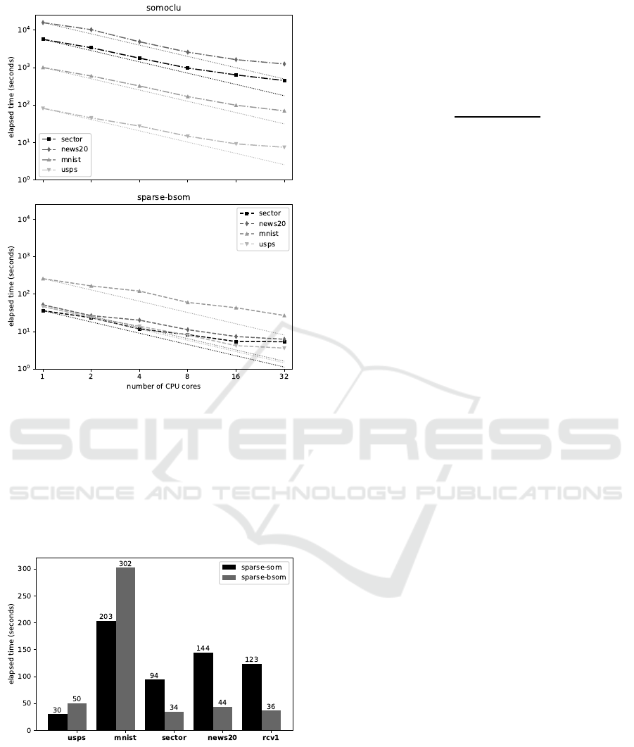
Figure 1: Parallel speed benchmark.
which is easy to explain, because this last algorithm
involves more calculations, and for this reason has
a larger constant factor in its time complexity. Less
clear is the reason why Sparse-Som performs better
on dense data. One possible interpretation is that it is
related to the different memory access management in
both algorithms.
Figure 2: Serial speed benchmark (lower is faster).
5.3 Quality Evaluation
Some authors have reported degradations in the re-
sulting maps using the batch algorithm (Fort et al.,
2002; N¨ocker et al., 2006). Here we look for such
effects with our implementations.
5.3.1 Methodology
Various metrics can be used to analyze the maps with-
out human labelling, the most common one is the av-
erage quantization error (Kohonen et al., 1996) de-
fined as
Q =
∑
N
i=1
kx
i
− w
c
k
N
(9)
where w
c
is the best match unit for x
i
.
Since SOM can be used in a supervised manner
to classify input vectors, one can also use standard
evaluation metrics (recall, precision). Because our
datasets are all multi-class, we calculate metrics for
each label, and find their average, weighted by sup-
port (the number of true instances for each label).
We have used the following evaluation method for
all datasets:
1. train the SOM network with the training part of
the dataset.
2. perform units calibration with the associated la-
bels (each unit is labeled according to the majority
of the data it matches).
3. predict the labels of the train data according to the
label attributed to their best match units.
4. do the same as step 3 on the test data.
If a unit has not attracted data in the training stage,
it is not labeled; if in test stage it attracts some in-
put data, we assign it a non-existent class. Though
this strategy can significantly decrease the overall re-
call score (it is possible to use more sophisticated ap-
proaches to deal with such cases), this simple method
is in general enough to analyze the clustering quality.
5.3.2 Results
Detailed results are shown in Table 2: Quantization
error and Table 3: Prediction evaluation (best F-score
highlighted). The experiments were run five times,
and we report mean values and standard deviation for
each system.
It should be emphasized that no parameters op-
timization per dataset was performed, and that it is
certainly possible to obtain better results with care-
ful parameter tuning. For example, the network we
have used (1200 units) is too large for small training
datasets, which probably explains the low recall rate
for the dna dataset. It seems, however, that the stan-
dard SOM version is more robust against such type of
difficulty, indicating that data samples are better dis-
tributed over the network with this algorithm.
The first observation we can make is that, though
not exactly identical, results of both batch versions

Table 2: Quantization error.
Sparse-Som Sparse-BSom Somoclu
rcv1 0.825± 0.001 0.816± 0.001 0.817± 0.004
news20 0.905± 0.000 0.901± 0.001 0.904± 0.001
sector 0.814± 0.001 0.772± 0.003 0.780± 0.011
mnist 4.400± 0.001 4.500± 0.008 4.512± 0.005
usps 3.333± 0.002 3.086± 0.006 3.117± 0.010
protein 2.451± 0.000 2.450± 0.001 2.452± 0.001
dna 4.452± 0.006 3.267± 0.042 3.272± 0.013
satimage 0.439± 0.001 0.377± 0.001 0.378± 0.002
letter 0.357± 0.001 0.345± 0.002 0.349± 0.002
Table 3: Prediction evaluation.
Sparse-Som Sparse-BSom Somoclu
precision recall precision recall precision recall
rcv1
train 79.2± 0.5 79.3 ± 0.6 81.3± 0.4 82.1± 0.3 81.2 ± 0.4 81.9± 0.5
test 73.7 ± 0.4 70.6± 0.5 76.6± 0.4 72.6± 0.5 75.6± 0.5 71.2± 0.8
news20
train 64.2± 0.5 62.8 ± 0.5 50.3± 0.9 49.6± 0.8 50.8 ± 1.6 50.3± 1.6
test 60.0± 1.7 55.4± 1.3 47.8 ± 1.2 43.6± 1.2 47.0± 1.9 42.8± 1.4
sector
train 77.2± 0.9 73.2 ± 0.9 58.4± 0.5 56.0± 1.0 57.3 ± 1.4 54.3± 3.1
test 73.3± 0.8 61.3± 1.8 60.9 ± 1.3 44.8± 1.0 60.5± 3.3 41.3± 3.6
mnist
train 93.5± 0.2 93.5 ± 0.2 91.5± 0.2 91.5± 0.2 91.3 ± 0.3 91.3± 0.3
test 93.4± 0.2 93.4± 0.2 91.7 ± 0.2 91.7± 0.2 91.7± 0.4 91.7± 0.4
usps
train 95.9± 0.2 95.9 ± 0.2 95.6± 0.2 95.6± 0.2 95.7 ± 0.2 95.7± 0.2
test 91.4 ± 0.3 90.7± 0.3 92.4± 0.5 91.5± 0.4 92.1± 0.5 91.3± 0.4
protein
train 56.7± 0.2 57.5 ± 0.2 56.7± 0.4 57.6± 0.3 56.3 ± 0.3 57.2± 0.2
test 49.8 ± 0.7 51.2± 0.6 50.7± 0.7 52.1± 0.6 50.5± 1.0 51.6± 0.5
dna
train 90.9± 0.6 90.8 ± 0.5 88.5± 0.6 88.5± 0.5 89.3 ± 0.6 89.3± 0.6
test 77.7± 1.5 69.6± 2.1 81.9 ± 2.9 30.3± 1.7 83.9± 2.7 25.1± 1.1
satimage
train 92.3± 0.4 92.4 ± 0.3 92.5± 0.4 92.6± 0.4 93.0± 0.2 93.1± 0.1
test 87.6 ± 0.3 85.4± 0.4 88.7± 0.5 86.3± 0.5 88.9± 0.3 85.5± 0.7
letter
train 83.8± 0.3 83.7 ± 0.3 81.9± 0.3 81.7± 0.4 81.3 ± 0.8 81.2± 0.8
test 81.5± 0.5 81.1± 0.5 80.2 ± 0.3 79.8± 0.5 78.9± 0.8 78.6± 0.8
(Somoclu and Sparse-BSom) are perfectly consis-
tent. Therefore, we focused our analysis on the dif-
ferences between our standard version and our batch
version.
With regard to the quantization error, it is clear
that the batch version performs better than the stan-
dard version, but this has no effect on the predictive
performance. The predictive benchmark results are
globally better with the standard version than with the
batch version. Furthermore, the results of the Sparse-
Som also seem to be more stable, and never fall much
lower than the Sparse-BSom results.
A significant gap occurs between the two versions
for the news20 and sector datasets, which are both
very sparse. However, we cannot generalize a nega-
tive impact of sparseness with the batch version, be-
cause of the counterexample with rcv1 results.
6 CONCLUSIONS
We have shown that, in case of the SOM algorithm,
the sparse nature of many data models can be ef-
fectively tackled using an appropriate formulation of
the calculations. The time required to train such
a network was reduced proportionally to the data
sparseness, and the input data can be used directly in
compressed form, which saves memory requirements.
This holds for both Sparse-Som and Sparse-BSom.
Sparse-BSom can also be parallelized efficiently
on multi-core CPUs, as demonstrated by our exper-
iments with OpenMP. This leads us to plan further
experiments on a cluster computing implementation,
potentially using MPI.
Unfortunately, due to the amount of synchroniza-
tion required, Sparse-Som is much harder to paral-

lelize, and we found no way to significantly improve
its performance compared to serial execution.
As regards the maps obtained with both our ver-
sions, we carried out an empirical qualitative analysis
using various datasets. Our results confirm the current
assumption that the behavior of the standard version
is more stable and generally produces overall better
results than the batch version.
In order to ensure reliable reproducibility
of our results, our complete implementation is
freely available online for the research commu-
nity, with its documentation, on GitHub, under
the terms of the GNU General Public License
(https://github.com/yoch/sparse-som).
ACKNOWLEDGEMENTS
We thank Gilles Bernard and Nourredine Aliane for
their valuable comments.
REFERENCES
Bandeira, N., Lobo, V., and Moura-Pires, F. (1998). Train-
ing a self-organizing map distributed on a pvm net-
work. In Neural Networks Proceedings, 1998. IEEE
World Congress on Computational Intelligence. The
1998 IEEE International Joint Conference on, vol-
ume 1, pages 457–461. IEEE.
Bernard, G., Aliane, N., and Manad, O. (2015). An exper-
imentation line for underlying graphemic properties -
acquiring knowledge from text data with self organiz-
ing maps. In ICINCO 2015 - Proceedings of the 12th
International Conference on Informatics in Control,
Automation and Robotics, Volume 1, Colmar, Alsace,
France, 21-23 July, 2015., pages 659–666.
Chang, C.-C. and Lin, C.-J. (2006). Libsvm data: Clas-
sification (multi class). https://www.csie.ntu.edu.tw/
∼cjlin/libsvmtools/datasets/multiclass.html.
Cheng, Y. (1997). Convergence and ordering of kohonen’s
batch map. Neural Computation, 9(8):1667–1676.
Dagum, L. and Menon, R. (1998). Openmp: an industry
standard api for shared-memory programming. IEEE
computational science and engineering, 5(1):46–55.
Fort, J.-C., Letremy, P., and Cottrell, M. (2002). Advantages
and drawbacks of the batch kohonen algorithm. In
ESANN, volume 2, pages 223–230.
Frey, P. W. and Slate, D. J. (1991). Letter recognition using
holland-style adaptive classifiers. Machine learning,
6(2):161–182.
Guan, H., Li, C.-k., Cheung, T.-y., and Yu, S. (1997). Paral-
lel design and implementation of som neural comput-
ing model in pvm environment of a distributed system.
In Advances in Parallel and Distributed Computing,
1997. Proceedings, pages 26–31. IEEE.
H¨am¨al¨ainen, T. D. (2002). Parallel implementation of self-
organizing maps. In Seiffert, U. and Jain, L. C., ed-
itors, Self-Organizing Neural Networks, pages 245–
278. Springer-Verlag, Inc., New York, USA.
Hull, J. J. (1994). A database for handwritten text recogni-
tion research. IEEE Transactions on pattern analysis
and machine intelligence, 16(5):550–554.
Ienne, P., Thiran, P., and Vassilas, N. (1997). Modified self-
organizing feature map algorithms for efficient digi-
tal hardware implementation. IEEE Transactions on
Neural Networks, 8(2):315–330.
King, R. D., Feng, C., and Sutherland, A. (1995). Stat-
log: comparison of classification algorithms on large
real-world problems. Applied Artificial Intelligence
an International Journal, 9(3):289–333.
Kohonen, T. (1982). Self-organized formation of topolog-
ically correct feature maps. Biological cybernetics,
43(1):59–69.
Kohonen, T. (1993). Things you haven’t heard about the
self-organizing map. In 1993 IEEE International Con-
ference on Neural Networks, pages 1147–1156. IEEE.
Kohonen, T. (1997). Self-Organizing Maps. Number 30
in Springer Series in Information Sciences. Springer,
second edition.
Kohonen, T. (2013). Essentials of the self-organizing map.
Neural Networks, 37:52–65.
Kohonen, T., Hynninen, J., Kangas, J., and Laaksonen, J.
(1996). Som pak: The self-organizing map program
package. Report A31, Helsinki University of Tech-
nology, Laboratory of Computer and Information Sci-
ence.
Kohonen, T., Kaski, S., Lagus, K., Salojarvi, J., Honkela, J.,
Paatero, V., and Saarela, A. (2000). Self organization
of a massive document collection. IEEE transactions
on neural networks, 11(3):574–585.
Lagus, K., Kaski, S., and Kohonen, T. (2004). Mining mas-
sive document collections by the websom method. In-
formation Sciences, 163(1):135–156.
Lang, K. (1995). Newsweeder: Learning to filter netnews.
In Proceedings of the 12th international conference on
machine learning, pages 331–339.
Lawrence, R. D., Almasi, G. S., and Rushmeier, H. E.
(1999). A scalable parallel algorithm for self-
organizing maps with applications to sparse data min-
ing problems. Data Mining and Knowledge Discov-
ery, 3(2):171–195.
LeCun, Y., Bottou, L., Bengio, Y., and Haffner, P. (1998).
Gradient-based learning applied to document recogni-
tion. Proceedings of the IEEE, 86(11):2278–2324.
Lewis, D. D., Yang, Y., Rose, T. G., and Li, F. (2004).
Rcv1: A new benchmark collection for text catego-
rization research. Journal of machine learning re-
search, 5(Apr):361–397.
Maiorana, F. (2008). Performance improvements of a
kohonen self organizing classification algorithm on
sparse data sets. In Proceedings of the 10th WSEAS
International Conference on Mathematical Methods,
Computational Techniques and Intelligent Systems,
MAMECTIS’08, pages 347–352. World Scientific
and Engineering Academy and Society (WSEAS).

McCallum, A. and Nigam, K. (1998). A comparison of
event models for naive bayes text classification. In
AAAI/ICML-98 Workshop on Learning for Text Cate-
gorization, Technical Report WS-98-05, pages 41–48.
Mulier, F. and Cherkassky, V. (1995). Self-organization as
an iterative kernel smoothing process. Neural compu-
tation, 7(6):1165–1177.
Natarajan, R. (1997). Exploratory data analysis in large,
sparse datasets. Technical report, IBMThomas J. Wat-
son Research Division.
N¨ocker, M., M¨orchen, F., and Ultsch, A. (2006). An algo-
rithm for fast and reliable esom learning. In ESANN,
14th European Symposium on Artificial Neural Net-
works, pages 131–136.
Noordewier, M. O., Towell, G. G., and Shavlik, J. W.
(1991). Training knowledge-based neural networks to
recognize genes in dna sequences. Advances in neural
information processing systems, 3:530–536.
Nordstr¨om, T. (1992). Designing parallel computers for self
organizing maps. In Proceedings of the 4th Swedish
Workshop on Computer System Architecture (DSA-
92), pages 13–15.
Seiffert, U. and Michaelis, B. (2001). Multi-dimensional
self-organizing maps on massively parallel hardware.
In Advances in Self-Organising Maps, pages 160–166.
Springer.
Silva, B. and Marques, N. (2007). A hybrid parallel som
algorithm for large maps in data-mining. New Trends
in Artificial Intelligence.
Tomsich, P., Rauber, A., and Merkl, D. (2000). Optimizing
the parsom neural network implementation for data
mining with distributed memory systems and cluster
computing. In Database and Expert Systems Appli-
cations, 2000. Proceedings. 11th International Work-
shop on, pages 661–665. IEEE.
Ultsch, A. (1999). Data mining and knowledge discovery
with emergent self-organizing feature maps for multi-
variate time series. Kohonen maps, 46:33–46.
Wang, J.-Y. (2002). Application of support vector machines
in bioinformatics. PhD thesis, National Taiwan Uni-
versity.
Wittek, P. (2013). Training emergent self-organizing maps
on sparse data with Somoclu. http://peterwittek.com/
training-emergent-self-organizing-maps-with-
somoclu.html.
Wittek, P., Gao, S. C., Lim, I. S., and Zhao, L. (2017). So-
moclu: An efficient parallel library for self-organizing
maps. Journal of Statistical Software, 78(9):1–21.
Wu, C.-H., Hodges, R. E., and Wang, C.-J. (1991). Par-
allelizing the self-organizing feature map on multi-
processor systems. Parallel Computing, 17(6-7):821–
832.
Yang, M.-H. and Ahuja, N. (1999). A data partition method
for parallel self-organizing map. In Neural Networks,
1999. IJCNN’99. International Joint Conference on,
volume 3, pages 1929–1933. IEEE.