Self-learning Smart Cameras

Harnessing the Generalization Capability of XCS

Anthony Stein

, Stefan Rudolph

, Sven Tomforde

and J

org H

ahner

Organic Computing Group, University of Augsburg, Eichleitnerstr 30, 86159 Augsburg, Germany

Intelligent Embedded Systems, University of Kassel, Wilhelmsh

oher Allee 73, 34121 Kassel, Germany

Keywords:

Organic Computing, Self-x, Self-learning, Self-adaptive, Reinforcement Learning, Smart Camera, Smart

Camera Network, Surveillance Camera, Learning Classiﬁer System, Extended Classiﬁer System, Q-learning.

Abstract:

In this paper, we show how an evolutionary rule-based machine learning technique can be applied to tackle

the task of self-conﬁguration of smart camera networks. More precisely, the Extended Classiﬁer System

(XCS) is utilized to learn a conﬁguration strategy for the pan, tilt, and zoom of smart cameras. Thereby,

we extend our previous approach, which is based on Q-Learning, by harnessing the generalization capability

of Learning Classiﬁer Systems (LCS), i.e. avoiding to separately approximate the quality of each possible

(re-)conﬁguration (action) in reaction to a certain situation (state). Instead, situations in which the same

reconﬁguration is adequate are grouped to one single rule. We demonstrate that our XCS-based approach

outperforms the Q-learning method on the basis of empirical evaluations on scenarios of different severity.

1 INTRODUCTION

The possible applications for networked cameras are

manifold (Hoffmann et al., 2008). The most common

use cases today are the detection of intruders in pri-

vate areas (e.g. the home of a person or research facil-

ities with classiﬁed prototypes) and the surveillance

of high risk areas (e.g the track area in train stations

or heavy machines in factories). But, there are also

future applications such as huge parking places where

the cameras could spot empty parking lots in order to

guide the drivers to them, or the monitoring of persons

that are potentially in need, such as nursing children

or ill people.

Today’s commercially available surveillance camera

systems consist of cameras with pan, tilt, zoom (PTZ)

capabilities. The captured video data is streamed to a

central control room where security staff tries to mon-

itor a large amount of this stream in parallel to identify

critical situations that require countermeasures. In

most cases, security staff is not able to fulﬁll this task

properly due to natural limitations in terms of han-

dling huge amounts of data simultaneously, e.g. mul-

tiple video streams at the same time, and the ability

to concentrate over long time, e.g. an entire working

day.

Previous work has addressed these issues by intro-

ducing smart cameras (Valera and Velastin, 2005).

These cameras include a computational unit that al-

lows to fulﬁll several tasks such as image process-

ing, photogrammetry, or object tracking. Intervention

of humans is optional, but not required for an efﬁ-

cient service of the system. Furthermore, most often

smart cameras form a network, resulting in a so-called

Smart Camera Network (SCN) (Rinner et al., 2008).

That introduces the additional challenge of coordina-

tion between the cameras. Such systems are mostly

designed to be self-organizing since they face the re-

quirement of only local interaction and decision mak-

ing since it is important to avoid problems that cannot

be computed in the given time limits or create huge

network loads. For example, in a huge smart cam-

era network, it is not possible to ﬁnd the globally best

alignment of all cameras in a short time span.

To enable a local decision making, Rudolph et al.

(2014) introduced the possibility of self-learning al-

gorithms for the alignment problem, i.e., to determine

the optimal PTZ conﬁguration for a certain situation.

Here, we pick this work up and improve their previous

results by introducing the Extended Classiﬁer System

(XCS) as control algorithm.

Accordingly, the contribution of this paper is the ap-

plication of a further, more sophisticated reinforce-

ment learning technique – the XCS – in order to im-

prove the self-learning capability of smart cameras.

Based on the results of the conducted studies, we also

Stein A., Rudolph S., Tomforde S. and HÃd’hner J.

Self-learning Smart Cameras - Harnessing the Generalization Capability of XCS.

DOI: 10.5220/0006512101290140

In Proceedings of the 9th International Joint Conference on Computational Intelligence (IJCCI 2017), pages 129-140

ISBN: 978-989-758-274-5

touch upon insights regarding the impacts of differ-

ent learning parameter conﬁgurations in scenarios of

varying complexity. Additionally, the resilience of the

techniques employed to equip smart cameras with the

intended self-learning capability is reﬂected in our ex-

periments by considering camera failures and look at

the time needed for the remaining camera to recover.

The remainder of this work is structured as follows:

In Section 2, we give an overview of related work in

the areas: (1) Coverage optimization in smart camera

networks, (2) applications of reinforcement learning

algorithms to smart cameras, and (3) the utilization

of Learning Classiﬁer Systems (LCS) (Holland et al.,

2000) in real world contexts. Subsequently, in Sec-

tion 3, we explain the general concept and learning

interaction of XCS, the most prominent representative

of LCS today. The formulation of our application sce-

nario as Markov Decision Process (MDP) and neces-

sary adaptions of the conventional XCS algorithm are

the subject of Section 4. We demonstrate the beneﬁt

of using XCS based on the results of conducted exper-

iments in Section 5. Eventually, Section 6 closes this

work with a brief summary and an outlook to planned

future work.

2 RELATED WORK

There are several works on the coverage optimiza-

tion of cameras (Sec. 2.1) and Reinforcement Learn-

ing (RL) in smart camera networks (Sec. 2.2). The

attempts include alignments through the PTZ capabil-

ities and the placement of the cameras. There are also

some works using RL techniques in the smart camera

domain. Furthermore, there are several real-world ap-

plications on which XCS has been applied (Sec. 2.3).

2.1 Coverage Optimization in SCN

Recently, (Liu et al., 2016) reviewed approaches for

the optimization of placement and alignment of cam-

eras. The majority of approaches focuses on settings

where a priori information about the environment is

available, e.g. the importance of particular spots.

Here, we follow a reinforcement learning approach,

i.e. the reconﬁgurations are based only on feedbacks

that we retrieve as a consequence of the realized ac-

tions (for a more detailed description of the reinforce-

ment learning approach, see Sec. 4.1).

Murray et al. (2007) focus on an urban model with po-

sitions that allow to install cameras. Then an off-line

optimization is used to determine the minimum num-

ber of cameras and the according alignment is calcu-

lated for the best coverage. This global optimization

is computationally highly intensive and therefore not

applicable for the on-line determination of the optimal

alignment that is in the focus of this work.

Erdem and Sclaroff (2006) propose a possibility to

optimize the placement and alignment of cameras ac-

cording to a given ﬂoor plan and task-speciﬁc con-

straints. The method proposed is an off-line optimiza-

tion algorithm and therefore can only be applied in ad-

vance to the camera installation. This paper focuses

on the optimization of the camera alignments during

runtime without previous knowledge of the environ-

ment.

Piciarelli et al. (2011) present an algorithm that uti-

lizes Expectation Maximization to optimize the align-

ment of coverage in a three dimensional environment,

but they focused on static and known environments.

2.2 Reinforcement Learning in SCN

Khan and Rinner (2012a) used Cooperative Q-

Learning to schedule tasks in a Wireless Sensor Net-

work and utilize it for an object tracking algorithm. In

following work (Khan and Rinner, 2012b), the same

authors employed artiﬁcial neural networks to tackle

the dynamic power management of a trafﬁc monitor-

ing system involving smart cameras among other sen-

sors.

Lewis et al. (2013) used bandit solvers as part of an al-

gorithm for the allocation of tracking objects to cam-

eras.

Even though RL techniques have been successfully

applied in the domain of smart camera networks, to

the best of our knowledge none of these contributions

focuses on the problem of camera alignment, except

for Rudolph et al. (2014). In this paper, we use one

particular approach presented in their work, the Q-

learning (Watkins and Dayan, 1992) algorithm, for

comparison purposes.

2.3 Learning Classiﬁer Systems in Real

World Scenarios

Learning Classiﬁer Systems (LCS) have gained

plenty of research attention since their invention by

John Holland (Holland, 1976). Initially designed to

solve binary encoded reinforcement learning tasks,

today many applications to real-world problems can

be found in the literature. For instance, Goldberg ap-

plied LCS to simulated gas pipeline control (Gold-

berg, 1987). An application to robot arm control was

reported by Stalph and Butz (2012).

Variants of LCS have been applied to system-on-chip

architectures in (Bernauer et al., 2011). Bull et al.

(2004) proposed the application of an LCS to trafﬁc

management. In Prothmann et al. (2008), a substan-

tially modiﬁed LCS that changes and constrains the

generalizing nature of the conventional system is pre-

sented and applied to adapt trafﬁc lights at urban in-

tersections.

What such real-world scenarios typically have in

common is the complexity of the underlying prob-

lem space. Not all possible states are known a priori

what necessitates learning during the system’s run-

time. Large problem spaces with complex reward

functions are the result. In consequence, the system

has to cope with unforeseen or not anticipated situa-

tions at runtime. In order to cope with this challenging

aspect, recently, a further extension was carried out to

XCS in Stein et al. (2017b). The incorporation of a

so-called interpolation component supports the sys-

tem by increasing the learning speed and reducing the

overall system error. This interpolation-based XCS

variant was also applied to the aforementioned trafﬁc

light management scenario in Stein et al. (2016).

Another application domain XCS was recently ap-

plied to, is the task of ensemble time series forecast-

ing. When signals are to be interpreted in techni-

cal systems, individual forecast methods have differ-

ent strengths and weaknesses for different character-

istics of time series. In Sommer et al. (2016a,b), an

XCS derivative for function approximation (XCSF)

was applied in order to learn the weights for a linear

combination of the outputs (forecast values) of a het-

erogeneous ensemble of forecasting techniques.

3 EXTENDED CLASSIFIER

SYSTEM

The Extended Classiﬁer System (XCS) is a ﬂexible,

evolutionary rule-based online machine learning sys-

tem. It was introduced in Wilson (1995) and can be

seen as one of the biggest milestones in LCS research.

XCS evolves its knowledge base as a population [P]

of condition-action rules, also called classiﬁers. This

set [P] is iteratively ﬁlled with a maximum number N

of classiﬁers of the following structure:

cl := (C, a, p, ε,F,exp,num,ts,as)

The ﬁrst attribute C determines a certain subspace

of the deﬁned n-dimensional state (or input) space

S that this classiﬁer covers and is called the condi-

tion. By this means, XCS partitions the state space

S into smaller subspaces. In contrast to tabular Q-

Learning (Watkins and Dayan, 1992) where for each

state-action pair a single Q-value is approximated

(more precisely |S × A| Q-values), XCS can general-

ize over a ﬁnite or even inﬁnite set of situations/states.

A classiﬁer cl is ‘activated’ and put to a so-called

match set [M] ⊆ [P] whenever a situation σ(t)

=~x ∈ S

arrives that is encompassed by the condition C of cl

(in the following we use the dot-notation to refer to

a speciﬁc attribute of a certain classiﬁer cl). cl.a ∈ A

represents one possible action of the action space A

that a speciﬁc classiﬁer cl advocates.

Each classiﬁer also maintains an incrementally calcu-

lated estimate of the average reward it has received

so far for advocating action a in one of the situations

σ ∈ cl.C which is usually called predicted payoff cl.p.

The mean absolute error of cl.p and the actually re-

ceived reward r after realizing action cl.a is stored

in the attribute cl.ε. The accuracy of predicting the

correct payoff relative to the environmental niche is

calculated as a sort of inverse of cl.ε and is called the

classiﬁer’s ﬁtness cl.F.

An experience statistic, cl.exp, gives indication of

how often this classiﬁer was selected for action exe-

cution and subsequently updated by the reinforcement

mechanisms of XCS.

The numerosity cl.num of a classiﬁer determines the

number of classiﬁers that this classiﬁer could sub-

sume so far. Subsumption happens when a classiﬁer

is found to be more or at least equally general as

another classiﬁer cl

which is to be subsumed. Addi-

tionally, cl

has to be more accurate than the prede-

ﬁned error tolerance ε

and must advocate the iden-

tical action as cl

. A classiﬁer with a cl.num > 1 is

called a macroclassiﬁer, whereas a newly generated

classiﬁer with cl.num == 1 is termed a microclassi-

ﬁer. The main advantage of introducing subsumption

to XCS is the reduced computational effort during the

matching procedure, as well as the more compact rep-

resentation of the entire population [P].

The so-called timestamp attribute cl.ts stores the last

time when the involved Genetic Algorithm (GA) was

invoked on a set of selected classiﬁers where this clas-

siﬁer also belonged to. It is used to control the appli-

cation frequency of the GA.

XCS attempts to create a maximally accurate, max-

imally general, complete and compact mapping S ×

A → R, where R determines the set of possible reward

values. To create a complete mapping, it is neces-

sary to guarantee that each environmental niche (sub-

space of the entire state space S) is covered and gets

assigned an equal amount of resources in terms of

microclassiﬁers. The action-set size attribute cl.as

is used to determine a deletion candidate classiﬁer

when the maximum number of microclassiﬁer N is

exceeded and thus the following condition holds:

∑

cl∈[P]

cl.num ≥ N. In consequence, each environ-

mental niche should have been assigned an equal

number of classiﬁers.

XCS is ﬂexible since it can be applied to a variety

of machine learning problems, e.g. Reinforcement

Learning problems (Wilson, 1995; Butz et al., 2005)

or rather Supervised Learning tasks, such as pure clas-

siﬁcation (Wilson, 2001) or also regression (Stalph

and Butz, 2012). There have also been investigations

on using XCS as an unsupervised learning mecha-

nism (Tamee et al., 2007).

XCS is called an evolutionary learning system since

it relies on a steady-state niche GA to ﬁnd a glob-

ally optimal state space coverage. The system thereby

pursues two main goals: (1) evolve classiﬁes that are

maximally general, and (2) retain maximal predic-

tion accuracy. This relationship in combination with

population-wide deletion became known as Wilson’s

generalization hypothesis (Wilson, 1995) and was ex-

tended by Kovacs to the optimality hypothesis (Ko-

vacs, 1998).

In essence, XCS learns in an online fashion by par-

titioning the state space S into smaller problems and

by estimating reward predictions locally by means of

(stochastic) gradient-descent techniques (Lanzi et al.,

2007). Additional to the local approximation, the in-

corporated GA is responsible for optimizing the state

space coverage globally. From an architectural point

of view, XCS can be decomposed into three main

components: (1) The performance component that

accomplishes the tasks of ﬁnding matching classi-

ﬁers and form [M], building the prediction array PA

that is further used to determine the action to be exe-

cuted a

exec

, and ﬁnally realizes the chosen action. (2)

The reinforcement component takes care of updating

all classiﬁers advocating the same action as the one

exec

) to be executed (these are grouped in a so-called

action set [A] ⊆ [M]) on the basis of the received re-

ward r ∈ R. (3) The discovery component comprises

the covering mechanism that is responsible for gener-

ating classiﬁers on demand, as well as the steady-state

niche GA for reﬁning the conditions of already exist-

ing classiﬁers to reach an optimal state space cover-

age.

4 APPROACH

This section describes our assumptions and deﬁnes

the problem space where the two algorithms under

consideration - XCS and Q-learning - are applied to.

Afterwards, we describe how XCS was adapted to ﬁt

the requirements of the outlined setting.

4.1 The Learning Task

We describe our Reinforcement Learning setting as

Markov decision process (MDP), see Sutton and

Barto (1998), and deﬁne the necessary components,

i.e. the state space S, the action space A, the reward

function r : S × A → R, as well as the state-transition

function δ: S × A → S.

4.1.1 State Space

The state of each smart camera controller is deﬁned

by the current values of its pan, tilt and zoom at-

tributes. Thus, the state can be described as a 3-

dimensional vector

s = (c

)

. We restricted the

set of possible values for c

according to reason-

able ranges and technical speciﬁcations. Furthermore,

we discretized the ranges as follows:

∈ {30, 60,.. .,360}, c

∈ {120, 150,180} and c

∈

{12,18}.

According to the above deﬁnitions, we get an state

space S with a magnitude of 12 · 3 · 2 = 72.

4.1.2 Action Space

For each of the three control variables that consti-

tute the state

s, a possible action determines whether

each of these values is increased (↑), decreased (↓)

or remains unchanged (=). This leads to an action

space A of a magnitude of 3 · 3 · 3 = 27. We prede-

ﬁned the increase as well as the decrease amount for

each of the three control variables. An action vec-

tor ~a can thus be represented by numeric values, e.g.

~a = (+20,−30,0)

. This allows a simple vector ad-

dition to yield the new system state

(cf. Sec. 4.1.4).

Combined with the state space, the overall problem

space consists of |S| × |A| = 1944 state-action combi-

nations. Q-learning builds-up a table for each of these

possibilities. By using XCS, we strive to harness its

generalization capability to summarize similar state-

action pairs into a single classiﬁer.

We want to note that the action space could be re-

stricted in a way so that there is no entry within the

Q-table for actions that would have no effect on the

succeeding state. For instance, when the zoom value

is at its maximum value and the smart camera con-

troller suggests to further increase the zoom, the al-

gorithm would not need to approximate these values

since they were already sorted out a priori by a human

expert. However, such a restriction was not applied in

this work.

A corresponding restriction of the action space has

also not been applied to XCS for two reasons: (1) We

intended to reduce the design-time effort and, thus,

the system’s engineer. (2) Such a restriction is not that

simple to implement, since XCS – roughly speaking

– creates a sort of Q-table in an online manner and

is designed to attempt the construction of a complete

solution map S×A → R. Nonetheless, future research

efforts are planned to address the introduction of ex-

actly such exploration constraints to XCS.

4.1.3 Reward Function

After an action has been realized and, subsequently,

the camera was reconﬁgured, a reward is calculated

by determining the sum of newly detected objects

within the vision area of all smart cameras. Hence,

the reward is highly stochastic, since it depends not

only on the conﬁguration of a single camera, but also

on the current conﬁguration of all other cameras in

the scenario under consideration. Naturally, it also

depends on the previous conﬁguration of the camera

and the number of undetected objects that were ex-

actly in that vision ﬁeld, i.e. objects that have already

been detected by any smart camera do not increase the

reward of the current step.

The stochastic nature of our reward function neces-

sitates an adaptive and incremental update procedure

to converge to nearly optimal (Q-)values describing

the utility of realizing action ~a in state

s. As we de-

scribe in the next section, we utilized the conventional

method to cope with stochastic reward functions – a

learning rate β which has been determined via various

parameter studies.

4.1.4 State Transition Function

The state transition function δ is given by a simple

vector addition of the current state vector

s ∈ S and

the selected action~a ∈ A. Thus, the next state is deter-

mined as

= (c

)

+(a

)

. In this work,

we do not consider uncertainty as a consequence of

noisy reconﬁgurations. This aspect constitutes a fur-

ther topic on our research agenda.

4.2 Adaptations to XCS

Since we are confronted with a discretized state space,

it seemed plausible to rely on a derivative of the con-

ventional XCS system that is capable of dealing with

numeric input values. In Wilson (2001), Wilson intro-

duced an extension to XCS for nominal inputs. The

condition is represented by so-called interval predi-

cates that determine a lower and an upper bound for

values accepted to satisfy the condition. In Wilson

(2000), XCS was further extended toward XCSR – an

XCS variant for real-valued input values.

For our problem scenario, we adopted Wilson’s tech-

niques by the following means: The condition is en-

coded by three interval predicates (l, u), one for each

control variable (c

). Since the state space is

discrete, we modiﬁed the covering and mutation op-

erators of XCS to reduce the search space complexity

to a reasonable level. Whenever XCS needs to cover a

situation not encountered so far, in a ﬁrst step the con-

dition of the new classiﬁer is set exactly to the current

state

s. Subsequently, the lower and upper bounds for

each of the i = 1 . . . 3 control variables are adapted as

follows:

= l

− r

·U (M

cov

) and u

= u

+ r

·U (M

cov

Thereby r

is a predeﬁned range that determines a

discrete step along each state space dimension. M

cov

is a multiplier and U(M

cov

) delivers a uniformly dis-

tributed random integer value between 1 and M

cov

A similar procedure is applied to the mutation opera-

tor of the GA utilized by XCS to ﬁnd a globally op-

timal coverage of the problem space. The only dif-

ference is that the step range for mutation m

and

the multiplier M

mut

differ from r

and M

cov

, respec-

tively. Furthermore, for mutation it is also permit-

ted that the lower bound is increased and the upper

bound is decreased, i.e. l

= l

± m

· U(M

mut

) and

= u

± m

·U (M

mut

). The sign is also selected at

random.

So far, our applied interval representation has one

considerable drawback: Yet, the step ranges r

and

are globally deﬁned for any dimension of the state

space S. This may lead to an over-sized classiﬁer

condition that does not exactly meet the possible dis-

crete values of the control variables as deﬁned in Sec-

tion 4.1.1. The elimination of this drawback is left for

future work.

5 EVALUATION

In this section, we elaborate on the results of our em-

pirical investigations that were carried out in the con-

text of our described smart camera application. We

chose this application domain for two reasons: (1)

We can compare to previous work in this applica-

tion context that adopts reinforcement learning tech-

niques (Rudolph et al., 2014). (2) SCNs provide a re-

alistic (real world) problem which is a ﬁeld of active

research (Piciarelli et al., 2016).

We conduct the experiments in a 3D simulation with

PTZ-capable cameras. The objective of the cameras

is to detect as many new objects as possible, i.e. al-

ready detected objects are not of interest. We explic-

itly note that the system goal is not congruent to the

coverage maximization, since depending on the setup

it is not necessary to observe the whole space but only

the regions that are populated with objects. Such an

objective is suitable, e.g. for a people counter in a

shopping mall, or for security purposes at the airport

(detecting wanted criminals).

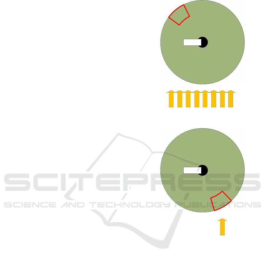
5.1 Experimental Setup

We compare the performance of XCS and Q-learning

in three different scenarios which are depicted in Fig-

ures 1, 2, and 3. The schematics show a top view.

Each scenario consists of one or multiple cameras

which are represented by a black dot. Around the

cameras, the colored sphere indicates the potential

observable space, i.e. the area that can be observed

when an appropriate PTZ-conﬁguration is assumed.

The small subregion – depicted by a red box – rep-

resents an exemplary ﬁeld of view. For clariﬁcation,

the entire colored sphere cannot be observed at once,

but only partially as indicated by the red boxed area.

Furthermore, the yellow arrows represent entry points

and the movement direction of the objects to be de-

tected. The quantity of entering objects is determined

by a probabilistic process that can be described as fol-

lows: Within a maximal interval of t

max

ticks an object

enters the scene every U(1,t

max

) ticks, where again

U(min, max) delivers a uniformly distributed random

integer between min and max.

Please note that the ﬁgures only provide a schematic

view on the different scenarios, but the actual ex-

periments have been conducted in a simulated 3-

dimensional environment.

Scenario 1. In this setting, one single camera in the

middle of the space is asked to observe as many ob-

jects as possible. The objects enter the scene from the

south. An adequate strategy for the camera would be

to alternate between several pan conﬁgurations, since

with a static conﬁguration it is not possible to reach a

high reward.

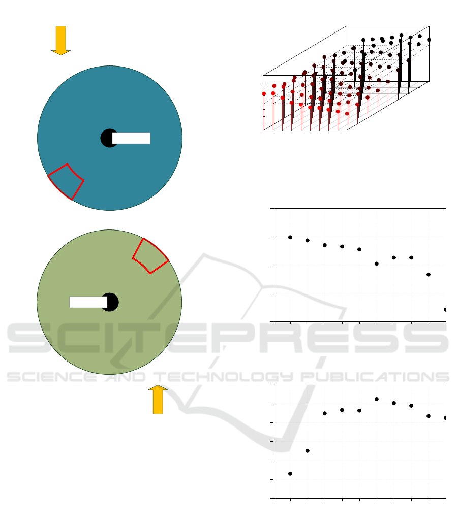
Scenario 2. In the second scenario, the number of

objects is signiﬁcantly decreased to one single stream.

An exemplary strategy that allows to detect all objects

would be to employ a static conﬁguration that covers

the stream.

Scenario 3. The third scenario is inspired by an air-

port where two man conveyors or escalators are sit-

uated beside each other but with different movement

directions. Thus, a representative adequate strategy

would be that each camera focuses on one stream of

objects at a time using a static conﬁguration as for sce-

nario 2. A further challenge is introduced by a camera

failure at a certain point in time. Accordingly, the re-

maining camera suddenly has to observe both streams

Camera

Figure 1: Schematic representation of scenario 1. One cam-

era observes multiple streams of objects.

Camera

Figure 2: Schematic representation of scenario 2. One cam-

era observes a single stream of objects.

and is thus forced to reconﬁgure to an alternating con-

ﬁguration.

5.2 Parameter Study

For our parameter studies, we repeated the experi-

ments for 10 independent runs. For Q-learning, we

conducted a comprehensive parameter study com-

prising parameters learning rate β (For the sake

of consistency, we denote the learning rate with β

as it is typically the case for XCS. In the stan-

dard literature for Q-learning, the learning rate is

usually denoted by α.) and the discount factor

γ for scenario 1. We tested the ranges of β ∈

{0.1,0.2, . . . , 1.0}, γ ∈ {0.1,0.2,. . . ,0.9}. Regard-

ing the exploration/exploitation trade-off, we utilized

Camera 1

Camera 2

Figure 3: Schematic representation of scenarios 3. Two

cameras observe two single streams of objects.

the ε-greedy action-selection strategy, where ε deter-

mines the probability of choosing a random action in-

stead of the action with the maximum Q-value. Fur-

ther results, not included in this work, showed that an

exploration rate ε = 0.05 is appropriate for this learn-

ing task, therefore we limited the presented results to

this value. The Q-values have been initialized with

0.005. Each conﬁguration was executed for 30.000

steps. Each point on the plots shows the average over

the entire 30.000 steps. To also capture the learning

speed, we furthermore analyzed the learning progress

to support our decisions (for the sake of brevity, these

plots are not included in this paper.).

Figure 4(a) depicts the results as a 3-dimensional

scatter plot. As Figure 4(a) shows, for scenario 1, the

best results have been achieved with a conﬁguration

of β = 0.7, γ = 0.9.

0.1 0.2 0.3 0.4 0.5 0.6 0.7 0.8 0.9 1.0

15.015.516.016.517.017.518.018.519.0

0.1

0.2

0.3

0.4

0.5

0.6

0.7

0.8

0.9

Learning rate β

Discount factor γ

Reward

(a) Scenario 1: Full parameter study of the learning rate β

and the discount factor γ

0.0 0.1 0.2 0.3 0.4 0.5 0.6 0.7 0.8 0.9 1.0

0.195

0.196

0.197

0.198

0.199

Learning rate β

Reward

(b) Scenario 2: Parameter study of the learning rate β

0.0 0.1 0.2 0.3 0.4 0.5 0.6 0.7 0.8 0.9 1.0

0.200

0.225

0.250

0.275

0.300

0.325

0.350

Learning rate β

Reward

Figure 4: Results of the conducted parameter studies.

Points in the plot correspond to the average reward values

of 30.000 learning steps.

For the second and third scenario, we restricted our

study to the learning rate β, since a comprehensive pa-

rameter study for each scenario is not viable due to the

enormous computational effort. Thus, we ﬁxed the

value for γ to 0.9, since we yielded this value in

our ﬁrst parameter study for scenario 1. Furthermore,

higher values for γ in general seemed to be legit, since

we are confronted with a multi-step problem. The re-

sults of the partial parameter study for the scenarios 2

and 3 can be found in Figures 4(b) and 4(c), respec-

tively. As can be seen, for the second scenario β = 0.1

and for scenario 3 β = 0.6 yield the best conﬁgura-

tions. These observations could be supported by our

analysis of the learning progress of all investigated

conﬁgurations of β.

5.3 Comparison of XCS and Q-learning

In the following, we compare Q-learning with XCS.

For the comparison, we use the best conﬁguration

found for Q-learning based on the results of the pa-

rameter study described above. Each comparison is

based on 30 independent runs with 30.000 steps for

each algorithm. A statistical analysis was carried out

considering a signiﬁcance level of 5% (α = 0.05). We

performed a Shapiro-Wilk-test combined with a vi-

sual inspection of the Quantile-Quantile-plots to ﬁg-

ure out whether the differences of the two samples

stem from a normally distributed population. To test

on variance homogeneity, an F-test was conducted.

Depending on the data properties of variance homo-

geneity and normal distribution, we decided for an ad-

equate test.

Since a comprehensive parameter study is not feasi-

ble due to the large number of dependent parameters,

we handcrafted our conﬁguration based on domain

knowledge. For our experiments, XCS was conﬁg-

ured as follows: N = 800, α = 0.1, γ = 0.9, ε = 0.05,

δ = 0.1, ν = 5, θ

= 12, ε

= 0.05, θ

mna

= |A| = 27,

del

= 50, θ

sub

= 50, χ = 0.8, µ = 0.04, p

ini

= 0.005,

ini

= 0.0, F

ini

= 0.01, r

= 0.1, m

= 0.05, M

mut

cov

= 3. For each scenario, the learning rate β has

been set to the values we yielded from the conducted

parameter studies described above. Thus, to provide

a comparability, we adopted the learning rate values

used for Q-learning for our XCS conﬁguration. For

more details regarding the meaning of the standard

XCS parameters, we refer to (Butz and Wilson, 2002;

Wilson, 2000).

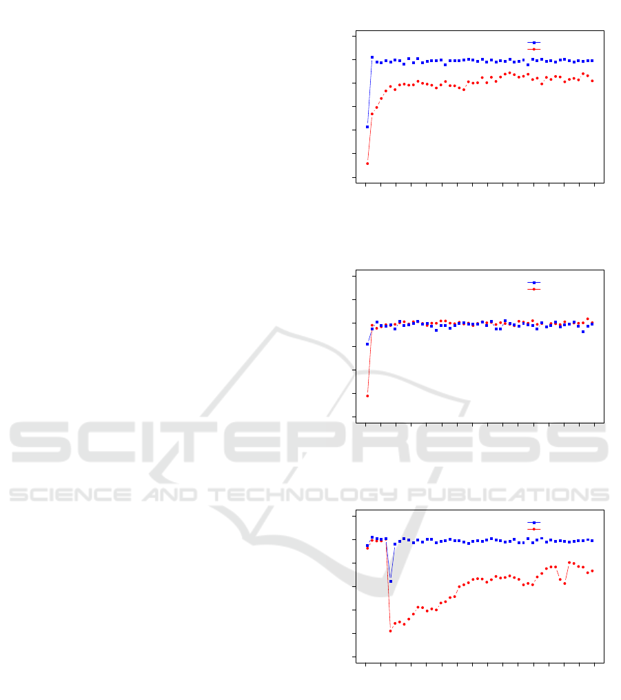
The results for scenario 1 can be found in Figure 5(a).

We see that XCS clearly outperforms Q-learning in

both learning speed and the quality of the learned

strategy. To compare the results of the two algo-

rithms in the overall performance, we relied on a

unpaired two sample t-test with signiﬁcance level

α = 0.05. XCS reached an overall reward of around

19.88 ± 0.05, whereas Q-learning showed an inferior

average performance of around 18.94 ± 0.27. The p-

value of the conducted two sample test is less than

Steps in 1000

Reward

0 2 4 6 8 10 12 14 16 18 20 22 24 26 28 30

XCS

Q−Learning

XCS vs. Q−Learning on Scenario 1

(a) Scenario 1, β = 0.7 for XCS and Q-learning

Steps in 1000

Reward

0 2 4 6 8 10 12 14 16 18 20 22 24 26 28 30

0.100

0.125

0.150

0.175

0.200

0.225

0.250

XCS

Q−Learning

XCS vs. Q−Learning on Scenario 2

(b) Scenario 2, β = 0.1 for XCS and Q-learning

Steps in 1000

Reward

0 2 4 6 8 10 12 14 16 18 20 22 24 26 28 30

0.15

0.20

0.25

0.30

0.35

0.40

0.45

XCS

Q−Learning

XCS vs. Q−Learning on Scenario 3

Figure 5: Graphical comparison of XCS and Q-learning on

three scenarios. Each point depicts the aggregated system

reward, averaged over 600 measurements.

2.2 × 10

−16

, which indicates that the average perfor-

mance of XCS is signiﬁcantly higher.

In scenario 2, we face a quite different situation. In

Figure 5(b), we see that the learned strategy is of simi-

lar quality. However, during the initial learning phase,

XCS shows a faster learning behavior. We conducted

the same signiﬁcance test as for scenario 1. The av-

erage performance of XCS is around 0.197 ± 0.003.

Q-learning reaches a performance value of about

0.198 ± 0.001. This difference is marginal, and with

a p-value of 0.2827 not signiﬁcant.

The results for scenario 3 are shown in Figure 5(c).

There, during the initial learning phase, we see a sim-

ilar behavior of XCS and Q-learning. At step 3000 the

performance drops noticeably. This can be attributed

to the simulated failure of one camera. Afterwards,

we see a very fast recovery of the XCS controlled

camera, but, the Q-learning controlled camera on the

other hand does only show a rather slow upwards

trend. The overall performance was about 0.40 ±

0.002 for XCS and 0.31 ± 0.037 for Q-learning, re-

spectively. As indicated by the conducted two sample

t-test, the difference of the performances are statisti-

cally signiﬁcant having a p-value of 5.891 × 10

−14

Concluding the results, we observe that overall XCS

clearly outperforms Q-learning. This becomes appar-

ent in scenarios 1 and 3. Especially, we ﬁgured out

that XCS shows its strengths in scenario 3, where the

self-learning cameras are asked to adapt to abruptly

changing circumstances, i.e. the failure of a camera.

Also in the second scenario, we observed a higher

learning speed during the initial learning phase in

comparison to Q-learning, but the eventually learned

strategies are on the same level.

The observed performance beneﬁts are attributed to

the generalizing nature of XCS. For the deﬁned MDP

(cf. Sec. 4.1), Q-learning has to individually approx-

imate |S × A| = 1944 state-action pairs within its Q-

table. XCS is able to yield improved results with only

≤ 800 (= N) macroclassiﬁers, each representing a

certain subset of the entire situation space S by means

of its interval encoding discussed in Section 4.2. This

leads to a simultaneous approximation of distinct but

adjacent state-action-pairs which in turn results in a

faster learning. The involved GA additionally exerts

evolutionary pressure toward an optimal coverage of

relevant subsets of the situation space S by favoring

the most accurate classiﬁers in the most frequently oc-

curring situations. A more proactive way of exploring

the situation space as proposed by Stein et al. (2017a)

could further improve the learning speed but is not

subject of this paper. Although the experimental re-

sults already show beneﬁts when using a generalizing

XCS, we assume that the performance difference can

still be increased when XCS is conﬁgured with nearly

optimal parameters. However, this necessitates an ex-

haustive parameter study which demands for a high

computational effort.

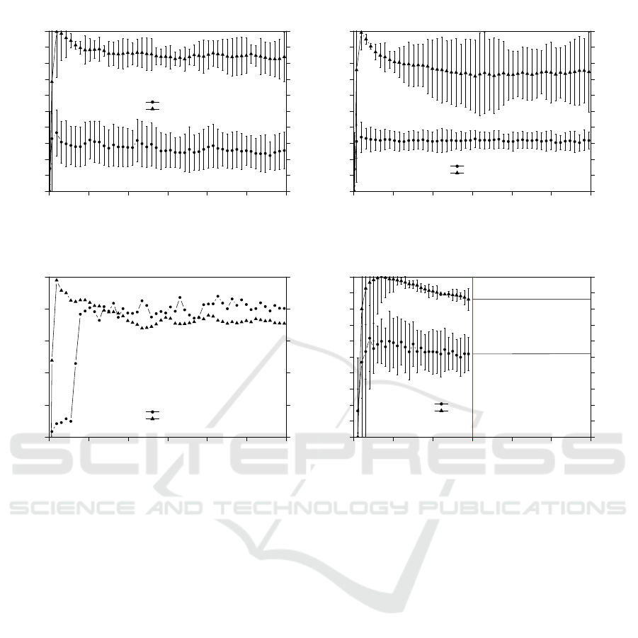
5.4 XCS Analysis

Figure 6 shows the learning progress of XCS. The

plots show two important metrics: (1) The mean abso-

lute system error, which averages the deviation from

the actual state-action value to the system prediction

over the last 100 steps. The system error relates to

the state-action value which comprises the reward for

realizing the chosen action of the previous step plus

the discounted maximum prediction array value of

the current time step. (2) The number of (macro-

)classiﬁers in the population [P], again averaged over

the last 100 steps.

As Figure 6(a) suggests, the system error in-

creases during the initial learning phase and subse-

quently decreases gradually. Considering the num-

ber of classiﬁers needed to approximate the problem

space, we can observe that after an initial peak near to

the allowed maximum number N, the level continu-

ously drops to less than 700 classiﬁers. Remembering

the superior performance of XCS in scenario 1, this is

a clear indicator that the utilization of XCS’ general-

ization mechanism yields beneﬁcial effects over the

tabular representation of Q-learning.

For the second scenario, on average we can observe

a more signiﬁcant decrease regarding the population

size |[P]|, however with a larger standard deviation

in comparison to scenario 1. This observation is at-

tributed to the fact that an optimal strategy for this

scenario appears to be much simpler than for the ﬁrst

scenario. Considering the system error, there is no

clear trend observable, i.e. the system error stagnates

on a similar level. Possible reasons for this behavior

are: (1) the stochastic nature of the reward function,

(2) the applied non-decaying probability of selecting

a random action ε = 0.05, as well as, (3) the restricted

expressiveness of the utilized interval condition rep-

resentation, as discussed in Section 4.2. Under the

presumption of the aforementioned error sources, we

expect that XCS has already converged to the minimal

achievable error (expected value).

The third scenario introduces a further challenge to

the system. After 3000 steps, we simulated a cam-

era failure. Both cameras deploy one XCS instance

each. During the initial phase before the camera fail-

ure, both cameras show a similar behavior regarding

the system error and the number of macroclassiﬁers in

the population (see Fig. 6(d)). Looking at Figure 6(c),

a sharp increase of the system error is observable sub-

sequent to the failure of the second camera. Subse-

quently, the system error oscillates and remains on

that increased level. As we outlined in Section 4.1,

the reward function of the present scenario is stochas-

tic. After the camera failure, the remaining camera

0 5000 10000 15000 20000 25000 30000

100

Steps

System Error

100

Macro Classifier

160

240

320

400

480

560

640

720

800

XCS System Error (+/− 1SD)

XCS Avg. Population Size (+/− 1SD)

XCS Performance on Scenario 1

(a) Scenario 1

0 5000 10000 15000 20000 25000 30000

0.0

0.2

0.4

0.6

0.8

1.0

Steps

System Error

0.0

0.1

0.2

0.3

0.4

0.5

0.6

0.7

0.8

0.9

1.0

Macro Classifier

160

240

320

400

480

560

640

720

800

XCS System Error (+/− 1SD)

XCS Avg. Population Size (+/− 1SD)

XCS Performance on Scenario 2

(b) Scenario 2

0 5000 10000 15000 20000 25000 30000

0.5

0.6

0.7

0.8

0.9

1.0

Steps

System Error

0.5

0.6

0.7

0.8

0.9

1.0

Macro Classifier

400

480

560

640

720

800

XCS System Error

XCS Avg. Population Size

XCS Performance on Scenario 3 for Camera 1

0 1000 2000 3000 4000 5000 6000

0.0

0.2

0.4

0.6

0.8

1.0

Steps

System Error

0.0

0.1

0.2

0.3

0.4

0.5

0.6

0.7

0.8

0.9

1.0

Macro Classifier

160

240

320

400

480

560

640

720

800

XCS System Error (+/− 1SD)

XCS Avg. Population Size (+/− 1SD)

XCS Performance on Scenario 3 for Camera 2

(d) Scenario 3 for broken camera 2

Figure 6: Learning progress of the XCS learning algorithm in terms of the number of evolved macroclassiﬁers and the system

error for the three considered scenarios. For the sake of readability, we omitted the error bars depicting the standard deviation

in subﬁgure (c).

is asked to observe both streams of objects to be de-

tected. Thus, more reward can be gained but the de-

gree of non-determinism also increases. As for sce-

nario 2, we assume that the error level has already

converged and can hardly decrease further due to the

aforementioned three reasons. As for the ﬁrst and the

second scenario, also in scenario 3 the average pop-

ulation size gradually reduces to a level of less than

700 classiﬁers.

6 CONCLUSION

Surveillance networks face certain challenges such

as ﬁnding the the optimal camera alignment or au-

tomated detection of suspicious events. In this paper,

we addressed the issue of automated camera align-

ment by means of reinforcement learning approaches

that aim to maximize the number of detected objects

in the observable range. We adapted the well-known

extended classiﬁer system technique and applied it to

the camera control problem. Within our experimen-

tal evaluation, we compared the approach to an alter-

native technique, the Q-learning algorithm, that has

been previously proposed for the same problem set-

ting in literature. We demonstrated that the XCS-

based approach is able to signiﬁcantly increase the

utility. This observation was attributed to the general-

ization approach of this particular learning system.

Future Work. As already indicated within the pa-

per, our current and future work focuses on two main

challenges resulting from the presented approach: (1)

an introduction of exploration constraints in XCS may

be beneﬁcial to guide the exploration behavior and

improve the learning speed, and (2) the incorporation

of expert knowledge (i.e. a priori knowledge of hu-

mans) may also be used to steer the desired learning

behavior. In addition, we will apply the developed

technique to large-scale simulation with hetero-

geneous constellations of cameras, e.g. in terms of

varying capabilities.

ACKNOWLEDGEMENTS

This research is partially funded by the DFG within

the project CYPHOC (HA 5480/3-2).

REFERENCES

Bernauer, A., Zeppenfeld, J., Bringmann, O., Herkersdorf,

A., and Rosenstiel, W. (2011). Combining Soft-

ware and Hardware LCS for Lightweight On-chip

Learning. In Organic Computing, pages 253–265.

Birkh

auser Verlag, Basel, CH.

Bull, L., Sha’Aban, J., Tomlinson, A., Addison, J., and Hey-

decker, B. (2004). Towards Distributed Adaptive Con-

trol for Road Trafﬁc Junction Signals using Learning

Classiﬁer Systems. In Bull, L., editor, Applications

of Learning Classiﬁer Systems, volume 150 of Stud-

ies in Fuzziness and Soft Computing, pages 276–299.

Springer Berlin Heidelberg.

Butz, M., Goldberg, D., and Lanzi, P. (2005). Gradi-

ent descent methods in learning classiﬁer systems:

improving XCS performance in multistep problems.

Evolutionary Computation, IEEE Transactions on,

9(5):452–473.

Butz, M. and Wilson, S. W. (2002). An Algorithmic De-

scription of XCS. Soft Comput., 6(3-4):144–153.

Erdem, U. M. and Sclaroff, S. (2006). Automated camera

layout to satisfy task-speciﬁc and ﬂoor plan-speciﬁc

coverage requirements. Computer Vision and Image

Understanding, 103(3):156–169.

Goldberg, D. E. (1987). Computer-aided pipeline opera-

tion using genetic algorithms and rule learning. part

ii: Rule learning control of a pipeline under normal

and abnormal conditions. Engineering with Comput-

ers, 3(1):47–58.

Hoffmann, M., H

ahner, J., and M

uller-Schloer, C. (2008).

Towards Self-organising Smart Camera Systems,

pages 220–231. Springer Berlin Heidelberg, Berlin,

Heidelberg.

Holland, J. H. (1976). Adaptation. In Rosen, R. and Snell,

F., editors, Progress in Theoretical Biology, volume 4,

pages 263–293. Academic Press, New York.

Holland, J. H., Booker, L. B., Colombetti, M., Dorigo, M.,

Goldberg, D. E., Forrest, S., Riolo, R. L., Smith, R. E.,

Lanzi, P. L., Stolzmann, W., and Wilson, S. W. (2000).

What Is a Learning Classiﬁer System?, pages 3–32.

Springer Berlin Heidelberg, Berlin, Heidelberg.

Khan, M. I. and Rinner, B. (2012a). Resource coordination

in wireless sensor networks by cooperative reinforce-

ment learning. In PerCom Workshops, pages 895–900.

IEEE.

Khan, U. A. and Rinner, B. (2012b). A reinforcement learn-

ing framework for dynamic power management of a

portable, multi-camera trafﬁc monitoring system. In

GreenCom, pages 557–564.

Kovacs, T. (1998). XCS Classiﬁer System Reliably Evolves

Accurate, Complete, and Minimal Representations for

Boolean Functions. In Chawdhry, P., Roy, R., and

Pant, R., editors, Soft Computing in Engineering De-

sign and Manufacturing, pages 59–68. Springer Lon-

don.

Lanzi, P. L., Loiacono, D., Wilson, S. W., and Goldberg,

D. E. (2007). Generalization in the XCSF Classiﬁer

System: Analysis, Improvement, and Extension. Evol.

Comput., 15(2):133–168.

Lewis, P. R., Esterle, L., Chandra, A., Rinner, B., and Yao,

X. (2013). Learning to be different: Heterogeneity

and efﬁciency in distributed smart camera networks.

In Proceedings of the 7th IEEE Conference on Self-

Adaptive and Self-Organizing Systems (SASO), pages

209–218. IEEE Press.

Liu, J., Sridharan, S., and Fookes, C. (2016). Recent

advances in camera planning for large area surveil-

lance: A comprehensive review. ACM Comput. Surv.,

49(1):6:1–6:37.

Murray, A. T., Kim, K., Davis, J. W., Machiraju, R., and

Parent, R. E. (2007). Coverage optimization to sup-

port security monitoring. Computers, Environment

and Urban Systems, 31(2):133–147.

Piciarelli, C., Esterle, L., Khan, A., Rinner, B., and Foresti,

G. L. (2016). Dynamic reconﬁguration in camera net-

works: A short survey. IEEE Transactions on Circuits

and Systems for Video Technology, 26(5):965–977.

Piciarelli, C., Micheloni, C., and Foresti, G. L. (2011). Au-

tomatic reconﬁguration of video sensor networks for

optimal 3d coverage. In 2011 Fifth ACM/IEEE Inter-

national Conference on Distributed Smart Cameras,

pages 1–6.

Prothmann, H., Rochner, F., Tomforde, S., Branke, J.,

uller-Schloer, C., and Schmeck, H. (2008). Organic

Control of Trafﬁc Lights, pages 219–233. Springer

Berlin Heidelberg, Berlin, Heidelberg.

Rinner, B., Winkler, T., Schriebl, W., Quaritsch, M., and

Wolf, W. (2008). The evolution from single to per-

vasive smart cameras. In Distributed Smart Cameras,

2008. ICDSC 2008. Second ACM/IEEE International

Conference on, pages 1–10.

Rudolph, S., Edenhofer, S., Tomforde, S., and H

ahner,

J. (2014). Reinforcement learning for coverage op-

timization through PTZ camera alignment in highly

dynamic environments. In Proceedings of the In-

ternational Conference on Distributed Smart Cam-

eras, ICDSC ’14, Venezia Mestre, Italy, November 4-

7, 2014, pages 19:1–19:6.

Sommer, M., Stein, A., and H

ahner, J. (2016a). Ensemble

Time Series Forecasting with XCSF. In 2016 IEEE

10th International Conference on Self-Adaptive and

Self-Organizing Systems (SASO), pages 150–151.

Sommer, M., Stein, A., and H

ahner, J. (2016b). Local en-

semble weighting in the context of time series fore-

casting using XCSF. In 2016 IEEE Symposium Series

on Computational Intelligence (SSCI), pages 1–8.

Stalph, P. O. and Butz, M. V. (2012). Learning local lin-

ear jacobians for ﬂexible and adaptive robot arm con-

trol. Genetic Programming and Evolvable Machines,

13(2):137–157.

Stein, A., Maier, R., and H

ahner, J. (2017a). Toward Cu-

rious Learning Classiﬁer Systems: Combining XCS

with Active Learning Concepts. In Proceedings of the

Genetic and Evolutionary Computation Conference

Companion, GECCO ’17, pages 1349–1356, New

York, NY, USA. ACM.

Stein, A., Rauh, D., Tomforde, S., and H

ahner, J. (2017b).

Interpolation in the eXtended Classiﬁer System: An

architectural perspective. Journal of Systems Archi-

tecture, 75:79 – 94.

Stein, A., Tomforde, S., Rauh, D., and H

ahner, J. (2016).

Dealing with Unforeseen Situations in the Context of

Self-Adaptive Urban Trafﬁc Control: How to Bridge

the Gap? In 2016 IEEE International Conference on

Autonomic Computing (ICAC), pages 167–172.

Sutton, R. and Barto, A. (1998). Reinforcement learning:

An introduction, volume 116. Cambridge University

Press.

Tamee, K., Bull, L., and Pinngern, O. (2007). Towards

Clustering with XCS. In Proceedings of the 9th An-

nual Conference on Genetic and Evolutionary Com-

putation, GECCO ’07, pages 1854–1860, New York,

NY, USA. ACM.

Valera, M. and Velastin, S. (2005). Intelligent distributed

surveillance systems: a review. Vision, Image and Sig-

nal Processing, IEE Proceedings -, 152(2):192–204.

Watkins, C. J. and Dayan, P. (1992). Q-learning. Machine

learning, 8(3):279–292.

Wilson, S. W. (1995). Classiﬁer Fitness Based on Accuracy.

Evolutionary Computation, 3(2):149–175.

Wilson, S. W. (2000). Get Real! XCS with Continuous-

Valued Inputss. In Lanzi, P. L., Stolzmann, W., and

Wilson, S. W., editors, Learning Classiﬁer Systems,

volume 1813 of Lecture Notes in Computer Science,

pages 209–219. Springer Berlin Heidelberg.

Wilson, S. W. (2001). Mining Oblique Data with XCS. In

Luca Lanzi, P., Stolzmann, W., and Wilson, S. W., edi-

tors, Advances in Learning Classiﬁer Systems, volume

1996 of Lecture Notes in Computer Science, pages

158–174. Springer Berlin Heidelberg.