Forecasting Time Series Data with Artificial Neural Network of

Bayesian Regularization

Doni El Rezen Purba

, Herman Mawengkang

and Tulus

Faculty of Computer Sciences and Information Technology, Universitas Sumatera Utara, Medan - Indonesia

Faculty of Mathematics and Natural Sciences, Universitas Sumatera Utara, Medan - Indonesia

Keywords: Data Mining, Forecasting, Optimization, Training Function.

Abstract: Forecasting or predicting future events is important to take into account in order for an activity to proceed

properly. Flights predict the weather forecast, the banking industry predicts the price of currency, the health

world predicts the disease, the retail business predicts total sales. prediction or forecasting of events is

calculated using past data, usually in the form of time series. Artificial neural networks are capable of

forecasting time-series data. Forecasting results with artificial neural network is influenced from the network

architecture model is determined, one of which determination of training function. Based on research

conducted by Aggarwal KK (et al 2005) and Murru & Rossini, R. (2016), using Bayesian regularization

training function in their research, this research uses the algorithm for time clock data forecasting process

with several model of layer count and number of neurons. The results obtained with the number of 3 layers

and each neuron of 36, 12, 6 for the best process performance, and the number of neurons 24, 12, 6 for the

shortest iteration process.

1 INTRODUCTION

Forecasting activities are widely used in various

areas. predict future events will greatly affect the

success of an activity. In the field of aviation, for

example, weather forecasting to anticipate failure in

flight. Predictions of possible severe weather

resulting in communication disturbances due to

storms, or the presence of cumulonimbus clouds that

could endanger the flight. In the retail business is also

so, conducted forecasting to estimate the increase or

decrease sales of a product in order to be done

anticipation to avoid losses.

Many methods can be used to do the forecasting.

Can use statistical models or with artificial neural

networks. Artificial neural networks are a method of

forecasting that is directed at a simple mathematical

model of the workings of the human brain. The

complex nonlinear relationship between response and

predictor variables (Hyndman Rob J. 2014). The

statistical model can be called by classical forecasting

methods and artificial neural networks called modern

forecasting methods. There is also a combination of

both to do the forecasting. (Medeiros, et.al., 2006).

Many research has been done to determine the

best model of artificial neural network architecture

(Aggarwal K.K, et.al 2005). Problems about the slow

process of training, the variety of existing data, the

increasing need for information from available data

and the increasingly sophisticated computing

equipment to improve the process of computer work.

The results of forecasting with neural network

motion are influenced based on the data form and the

network architecture parameters used. The choice of

neural network model must be in accordance with the

form of data to be used. Vhatkar. S and Dias. J (2016)

conducted a research method of artificial

backpropagation network to forecast sales of oral care

products ranging from suppliers to final consumers to

help in determining business decisions. Zhao K. and

Wang C. (2017) used the Convolutional Neural

Network (CNN) model on his research on sales

forecasts in the E-commerce field using promotional

history data, price changes and user preferences to

help manage the workforce, cash flow and sources

power on the company based on the results of

forecasting done.

The selection of network models influences the

outcomes of the learning process, both the accuracy

of the results and the length of the calculation process.

Selection of activation functions, training functions

and the number of layers and neurons for the training

564

Rezen Purba, D., Mawengkang, H. and Tulus, .

Forecasting Time Series Data with Artiﬁcial Neural Network of Bayesian Regularization.

DOI: 10.5220/0010046505640568

In Proceedings of the 3rd International Conference of Computer, Environment, Agriculture, Social Science, Health Science, Engineering and Technology (ICEST 2018), pages 564-568

ISBN: 978-989-758-496-1

and testing process should be well considered.

Aggarwal K.K. (et al 2005) conducted a study titled

Bayesian Regularization in a Neural Network Model

to Estimate Lines of Code Using Function Points,

stating that, the neural network model trained using

Bayesian Regularization gave the best results and was

suitable for the study. Then, doing research on the

Effects of Training Functions of Artificial Neural

Networks (ANN) on Time Series Forecasting,

obtained from all the training algorithms used for

hourly weather history data forecasting, levenberg

marquardt proved to have the least squares error and

correlation coefficient (Aggarwal R and Kumar R.

2015).

Based on the exposure, in this research will be

conducted research for testing the best neural network

model against some time series data that has been

provided. To get the best forecasting results.

2 METHODS

2.1 Forecasting

Forecasting is the process of estimating future needs

that include the need for quantity, quality, time and

location required to meet the demand for goods or

services (Nasution, 1999).

Demand forecast is the level of demand for

products that are expected to be realized for a certain

period of time in the future. Basically the approach of

forecasting can be classified into two approaches,

namely (Makridakis, et.al., 1995):

1. Qualitative Forecasting

2. Quantitative Forecasting

There are 4 types of data patterns in forecasting

(Makridakis, et.al., 1995) :

1. Trend : The trend data pattern shows the

movement of data tends to increase or decrease

for a long time.

2. Seasonality : Seasonal data patterns are formed

due to seasonal factors, such as weather and

holidays.

3. Cycles : Cycle data patterns occur when

variations of corrugated data over a duration of

more than one year are influenced by political

factors, economic changes (expansion or

contraction), known as business cycles.

4. Horizontal/Stasionary/Random variation : This

pattern occurs if the data fluctuates around a

random average value without forming a clear

pattern such as a seasonal pattern, trend or cycle.

2.2 Neural Nerwork

An artificial neural network processes large amounts

of information in parallel and distributed, this is

inspired by the biological brain work model.

Hecht-Nielsend (1988) defines artificial neural

systems as: a distributed and parallel processed

information processing structure, consisting of a

processing element (which has local memory and

operates with local information) interconnected along

with a direct-line flow called a connection. Each

processor element has a single outlet connection that

fan out to the desired number of collateral

connections (each connection carrying the same

signal from the output of the processing element). The

output of the processing element can be any kind of

mathematical equation desired. The entire process

that takes place on each processor element must really

be done locally, ie the output depends only on the

input value at that moment obtained through the

connection and the value stored in the local memory.

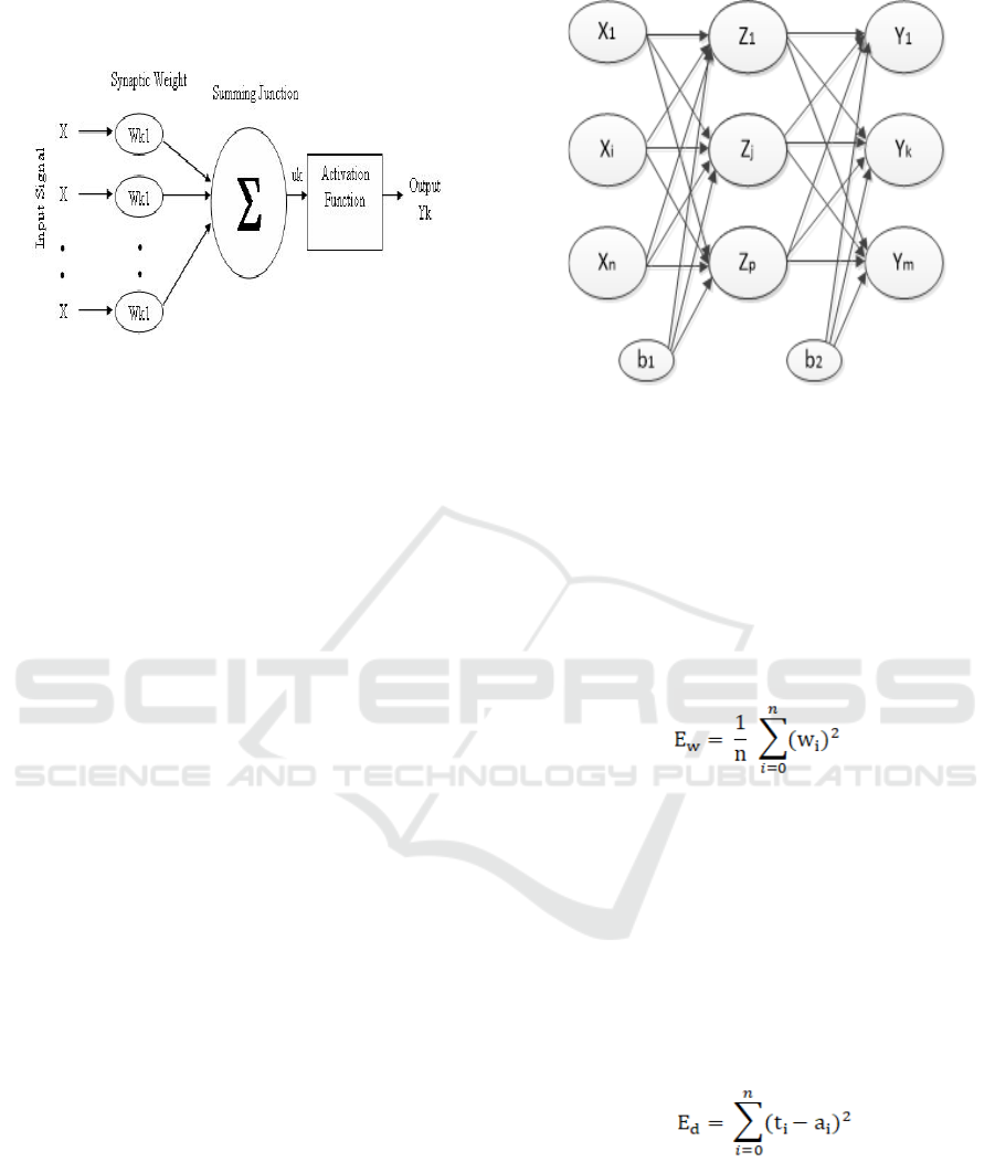
The structure in Figure. 1 is the basic standard

form of a unit of simplified human brain network

units. The human brain tissue is composed of 10

neurons connected by about 10

dendrites. The

dendrite function is as a transmitter of signals from

the neuron to the neurons connected to it. Nucleus is

the nucleus of a neuron, the axon acts as the output

channel of the neuron, and the synapses that govern

the strength of the relationship between neurons.

Figure 1. Structure of neural network biology

An artificial neural network consists of a collection of

neuron groups arranged in layers.

Forecasting Time Series Data with Artiﬁcial Neural Network of Bayesian Regularization

565

 Input Layer: serves as a network link to the

outside world (data source).

Figure 2. Structure of artificial neural network

 Hidden Layer: A network can have more than one

hidden layer or even can not have it at all.

 Output Layer: The working principle of neurons

in this layer is similar to the working principle of

neurons in the hidden layer and here also the

Sigmoid function is used, but the output of the

neurons in this layer is considered to be the result

of the process.

2.3 General Type of Neural Network

In general, there are three types of neural networks

that are often used based on the type of network it is:

 Single-Layer Neural is a neural network that has

connections on its input directly to the output

network.

 Multilayer Perceptron Neural Network is a neural

network that has a layer called "hidden", in the

middle of the input and output layers. Hidden is

variable, can be used more than one hidden layer.

 Recurrent Neural Networks Neural network is a

neural network that has characteristics, namely

the existence of a feedback connection from the

output to the input.

2.4 Backpropagation Neural Network

Backpropagation is one of the training methods of

Artificial Neural Network. Backpropagation uses a

multilayer architecture with supervised training

training methods. The Back Propagation Model has

several units that exist in one or more hidden layers.

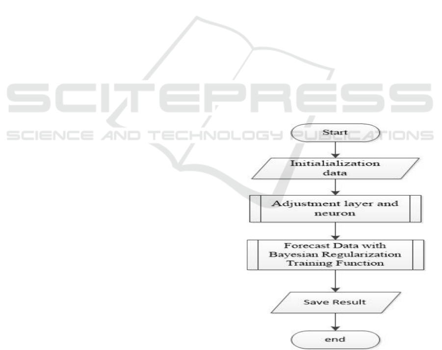
Figure 3 is a back propagation model architecture

with n input (plus one bias), a hidden layer consisting

of p units (plus a bias) and m units of output units.

Figure 3. Architecture of backpropagation neural network

2.5 Bayesian Regularization Algorithm

Regularization plays a role in improving the

generalization process by limiting the size of the

weight of a network. If the value of network weight is

smaller then the network will respond more subtly.

With regularization, a large, simplified network must

be able to represent the actual function. In the classic

Backpropagation algorithm it aims to minimize

functionality F=E

, where :

In this case n is the number of inputs in the

training set, t

is the target value in the data to-i and a

is the output for the data to-i which is obtained as a

neural network response.

The regulatory method changes the performance

of the error function by adding a standard deviation

of the weights and biases:

F = βE

+ αE

αβ is regularization parameter, and E

define as:

is a weight or a threshold. Using the equation

to change the error performance function allows the

network to obtain the smallest weights and

thresholds, but it can not determine effective network

weight and thresholds. The conventional method is

often difficult to determine the size of the parameter,

Mackay (1992) proposes a network that can adjust the

size of adaptive parameters using Bayesian

ICEST 2018 - 3rd International Conference of Computer, Environment, Agriculture, Social Science, Health Science, Engineering and

Technology

566

theoretical framework, and enables achievement of

optimal performance.

2.6 Backpropagation Neural Network

Forecasting

At the feed-forward stage, each input unit (X

)

receives the input signal and sends this signal to each

hidden unit Z1, ..., Zp. Each hidden unit counts its

activation and sends its signal (Z

) to each output unit.

Each output unit (Y

) calculates its activation (Y

) to

indicate the network response to the given input

pattern.

During the training, for each unit of output

compared to Yk activation with the target Tk to

determine the error between the input pattern and the

output unit. After obtained error value, factor δ

(k=1,...,m) calculated δ

which is used to distribute

the error on the Y

output unit back to all units on the

previous layer (hidden unit connected to Y

). Then

this error is used to change the weights between the

output and the layer with the hidden layer. In the same

way, the factor δ

(j=1,...,p) is calculated for each unit

. Factor δ

used to change the weights between the

hidden layers and the input layer.

After all the factors δ are determined, the weights

for the whole layer are adjusted directly. The weight

adjustment Wjk (from hideen unit Z

to Y

output

unit) is based on the factor δ

and activation of unit Z

The weight adjustment of the vij (from the X

input

unit hidden unit Z

) is based on the factor δ

and

activation of teh input unit x

The usual activation function used to train

artificial neural network is sigmoid function, both

binary and bipolar. Here's the training algorithm

(Fausett, Laurene, 1994) :

Step 0. Initialize initial weights (specifies a small

random value)

Step 1. As long as the stop condition is false, take

steps 2-9

Step 2. For each pair of training, step 3-8

(Feedforward)

Step 3. Each input unit (X

, i = 1, ... n) receives the

input signal X

and sends the signal throughout the

unit on the next layer (hidden layer).

Step 4. For each hidden unit (Z

, j = 1, ..., p), the input

signal is weighted in and applied the activation

function to calculate its output and send this signal to

all subsequent layer units (output layer).

Step 5. For each Output unit (Y

, k = 1, ..., m) see the

weighted input in sequence.

Back Propagation from Error

Step 6. For each output unit (Yk, k = 1, ..., m)

received a target pattern corresponding to the input

pattern, calculated the error and calculated the weight

correction and calculated the correction and sent δk to

the unit in the previous layer.

Step 7. For each hidden unit (Z

, j = 1, ..., p), the

summed delta function is then multiplied by its

activation function to calculate, calculated its weight

correction and correction.

Step 8. For each output unit (Yk, k = 1, ..., m) the bias

and weights are changed (j = 1, ..., p). For each hidden

unit (Z

, j = 1, ..., p) the weight and bias are changed

(i = 1, ..., p).

3 RESULT AND DISCUSSION

In this study used time series data of the population

of a region in Indonesia for the forecasting process.

The training function used is Bayesian

Regularization. The best network model is

determined based on the accuracy and speed of the

forecasting process. Prediction will be done by trying

some models of the number of layers and the number

of neurons. Table 1 below is a form of network model

that will be used for forecasting.

Figure 4. is flow diagram proses forecasting data

Forecasting Time Series Data with Artiﬁcial Neural Network of Bayesian Regularization

567

Table 1. The number of layers and the number of neurons

Model

umber of neurons

er 1 La

er 2 La

er 3

1 12 6 2

2 24 12 6

3 36 12 6

4 48 12 6

5 48 24 12

The program used for forecasting process in this

research is matlab. Source code as follows:

rng('default')

inputs = data_latih;

targets = target_latih;

x1 = number of neurol layer 1

x2 = number of neurol layer 2

x3 = number of neurol layer 3

net = newff(inputs,targets, { x1, x2,

x3});

net = train(net,inputs,targets);

net.trainFcn = 'trainbr';

outputs = net(inputs);

errors = outputs - targets;

perf = perform(net,outputs,targets)

figure,

plot(outputs,'bo-')

hold on

plot(targets,'ro-')

hold off

grid on

title(strcat(['Plot Performa NNBR,

Value = ', num2str(perf)]))

xlabel('Month -')

ylabel('Total Population')

legend('Output Neural Net','

Target','Location','Best')

figure,

plotregression(targets,outputs,'Regress

ion')

the results of data experiments with the network

model in Table 1 are presented in table 2.

Table 2. Result experiment

Model Result

iteration Perform Regresion

1 8 0.00094869 0.83259

2 7 0.00076587 0.83968

3 10 0.00046405 0.94414

4 7 0.0021427 0.3515

5 9 0.00081544 0.82761

4 CONCLUSIONS

From the result of research can be concluded that:

- Artificial neural network with training function

Bayesian Regularization can do well forecasting

- Best performance results are designated by

neural net 3 model but require more repetition

- The network model 2 is capable of converging

with less iteration and less bad performance

values

- Speed and performance are necessities that can

not be clearly compared. Both of these depend

on user requirements.

REFERENCES

Aggarwal K.K. , Singh Y, Chandra P and Puri P (2005),

Journal of Computer Sciences. Bayesian

Regularization in a Neural Network Model to Estimate

Lines of Code Using Function Points.

Aggarwal R and Kumar R. (2015). International Journal of

Computer Applications. Effect of Training Functions of

Artificial Neural Networks (ANN) on Time Series

Forecasting

Omar Hani, Hoang Van Hai, and Liu Duen-Ren. 2016.

Computational Intelligence and Neuroscience.

Hindawi Publishing Corporation.

Hyndman Rob J. 2014. The book, Forecasting: Principles &

Practice.

Masduqi, A., & Apriliani, E. 2008. Estimation of Surabaya

River Water Quality Using Kalman Filter Algorithm.

IPTEK, The Journal for Technology and Science, 19(3),

87–91.

Monjoly S, Andre M, Calif R, Soubdhan T. 2017. Hourly

forecasting of global solar radiation based on

multiscale decomposition methods: A hybrid approach.

International Journal Of Energy : Vol. 119 : 288-298.

https://doi.org/10.1016/j.energy.2016.11.061

Murru, N., & Rossini, R. 2016. Neurocomputing A

Bayesian approach for initialization of weights in

backpropagation neural net with application to

character recognition. Neurocomputing, 193, 92–105

ICEST 2018 - 3rd International Conference of Computer, Environment, Agriculture, Social Science, Health Science, Engineering and

Technology

568