Deep Learning versus Gist Descriptors for Image-based Malware

Classiﬁcation

Sravani Yajamanam, Vikash Raja Samuel Selvin, Fabio Di Troia and Mark Stamp

Department of Computer Science, San Jose State University, San Jose, California, U.S.A.

Keywords:

Malware Detection, Gist Descriptors, Support Vector Machine, k-nearest Neighbor, Deep Learning, Ten-

sorFlow.

Abstract:

Image features known as “gist descriptors” have recently been applied to the malware classiﬁcation problem.

In this research, we implement, test, and analyze a malware score based on gist descriptors, and verify that

the resulting score yields very strong classiﬁcation results. We also analyze the robustness of this gist-based

scoring technique when applied to obfuscated malware, and we perform feature reduction to determine a

minimal set of gist features. Then we compare the effectiveness of a deep learning technique to this gist-based

approach. While scoring based on gist descriptors is effective, we show that our deep learning technique

performs equally well. A potential advantage of the deep learning approach is that there is no need to extract

the gist features when training or scoring.

1 INTRODUCTION

In this research, we apply techniques from the dom-

ain of image processing to the malware classiﬁcation

problem. The underlying idea is to treat malware bi-

naries as images and classify the samples based on

properties of the resulting images.

As the name suggests, a “gist” descriptor pro-

vides a high-level—and hence, low-dimensional—

representation of some important aspect of an image.

Gist descriptors are designed to match human con-

cepts with respect to various features of images. Intui-

tively, when used in malware analysis, gist descriptors

can enable us to see the “big picture,” so that we can

ignore minor variations and obfuscations that invaria-

bly occur within a malware family. That is, from the

high level perspective of gist descriptors, differences

within families will likely appear negligible in com-

parison to the differences between families. Techni-

ques that rely on a more detailed perspective (e.g.,

statistical analysis based on opcodes) might be more

easily defeated by the “noise” that exists within a mal-

ware family, particularly malware that is intentionally

obfuscated in some reasonably sophisticated way.

The remainder of this paper is structured as fol-

lows. In Section 2 we brieﬂy discuss relevant back-

ground topics. Then in Section 3 we give our main

experimental results. In these experiments, we ana-

lyze the strength and robustness of a malware classiﬁ-

cation technique that relies on gist descriptors as fea-

tures. For comparison, we also consider experiments

involving deep learning techniques based on the same

dataset of malware images, but without using gist des-

criptors. Section 4 concludes the paper and provides

suggestions for future work.

2 BACKGROUND

In practice, the most popular method of malware de-

tection is signature scanning, whereby pattern mat-

ching is used to detect speciﬁc signatures that have

been previously extracted from known malware sam-

ples. While signature scanning can be highly ef-

fective, such an approach can be defeated by making

minor modiﬁcations to malware, as such code modi-

ﬁcations will often break existing signatures.

Statistical and machine learning based malware

detection techniques are signiﬁcantly more robust

than standard signatures, yet these approaches have

also been shown to be susceptible to code obfuscati-

ons that alter various statistical or structural proper-

ties of malware samples. Thus, a critically important

problem in malware research is to ﬁnd efﬁcient and

practical methods that provide strong results, and yet

are robust in the face of obfuscation techniques that

can be easily employed by malware writers (Bayer

et al., 2006; Moser et al., 2007; Sharif et al., 2008;

Yajamanam S., Selvin V., Di Troia F. and Stamp M.

Deep Learning versus Gist Descriptors for Image-based Malware Classiﬁcation.

DOI: 10.5220/0006685805530561

In Proceedings of the 4th International Conference on Information Systems Security and Privacy (ICISSP 2018), pages 553-561

ISBN: 978-989-758-282-0

You and Yim, 2010).

Image processing techniques have been suggested

as the basis for malware scoring. In such scoring

techniques, we visualize malware binaries as grays-

cale images and attempt to classify malware samples

based on image properties.

The motivation (and starting point) for the work

presented here is the paper (Nataraj et al., 2011),

where high-level image features known as “gist des-

criptors” are used to successfully classify malware.

Here, we analyze the strength and robustness of gist-

based malware classiﬁcation, and we compare these

results to an image-based deep learning technique that

does not employ gist descriptors.

2.1 Gist Descriptors

In (Oliva and Torralba, 2001), Oliva and Torralba dis-

cuss a method for constructing a “spatial envelope” of

a scene or image in terms of various properties such

as “naturalness” and “openness.” These properties—

which are shown to be meaningful to humans—are

designed to capture the “gist” or essence of an image

by providing a connection between visual and seman-

tic information. The research in (Oliva and Torralba,

2001) is focused on the challenging problem of com-

puter vision.

Gist descriptors have proven useful in a wide vari-

ety of applications including, for example, web-scale

image search (Douze et al., 2009). A recent arti-

cle (Nataraj et al., 2011) shows that gist descriptors

can be used as the basis for an effective image-based

malware score. Speciﬁcally, the paper (Nataraj et al.,

2011) (which, as mentioned above, is the motivation

for our research here) claims to classify malware va-

riants belonging to 25 different families with an im-

pressive accuracy of almost 98%.

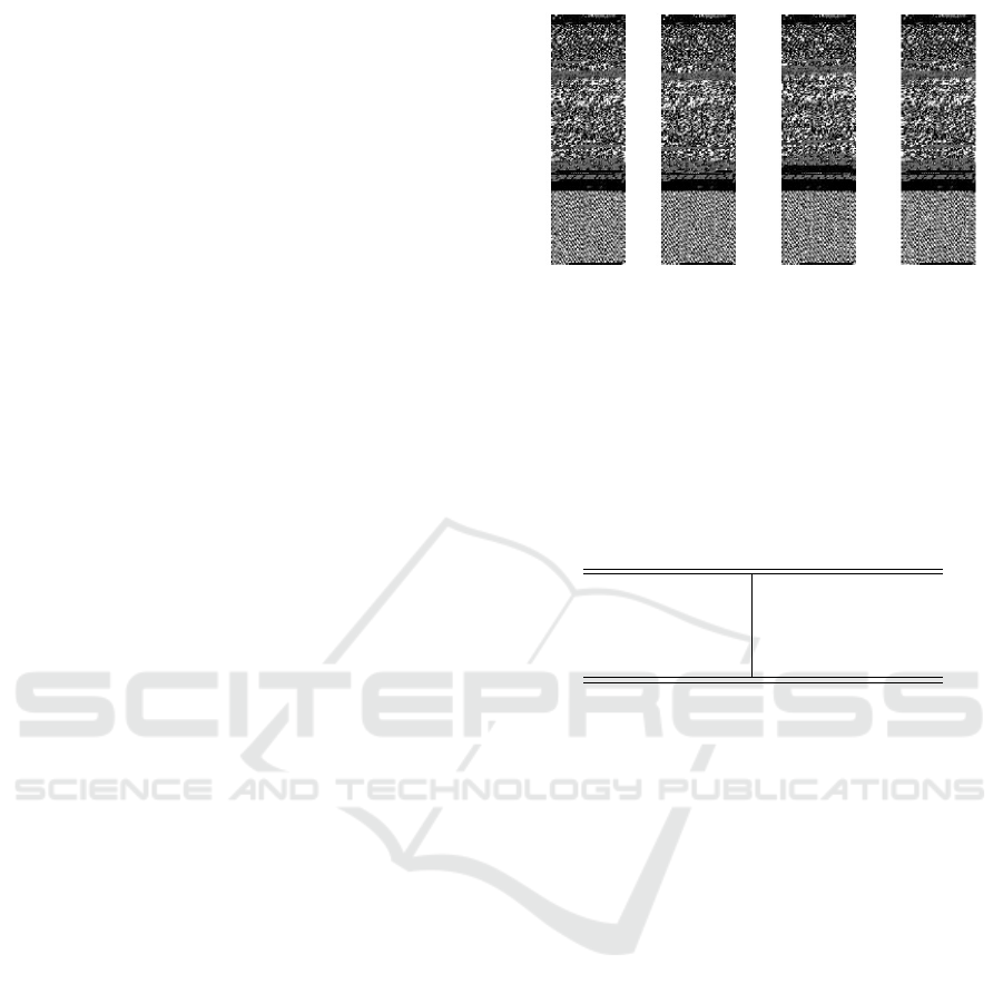
Figure 1 shows four variants of the malware fa-

mily Dialplatform.B viewed as images. In this case,

we clearly see common structure in the images, which

indicates there is signiﬁcant potential for an image-

based malware scoring technique.

3 EXPERIMENTS AND RESULTS

In this section, we discuss our experimental design

and we provide a selection of our results. Additio-

nal related results can be found in the report (Selvin,

2017).

Figure 1: Variants of the malware family Dialplatform.B

viewed as images.

3.1 Implementation Details

To conduct the various experiments discussed in this

paper, we used the software, hardware, and datasets

listed in Table 1. The Malimg and Malicia datasets

are discussed in the next section.

Table 1: Experimental Setup.

OS Ubuntu 14.04

Python version 2.7

Python libraries numpy, tensorﬂow

Datasets Malimg, Malicia

3.2 Datasets

A dataset known as Malimg formed the basis for the

experiments reported in (Nataraj et al., 2011), and we

use this same dataset here. The Malimg data consists

of more than 9000 malware samples belonging to 25

families. Table 2 lists the various families and num-

ber of samples in each family within the Malimg da-

taset. All of these malware binaries were treated as

images and all 320 gist features were extracted from

each sample. We have used the same image characte-

ristics (e.g., height and width) and the same gist des-

criptors as was used in the paper (Nataraj et al., 2011),

and hence our results are directly comparable.

We have also tested this gist-based scoring techni-

que on the challenging Malicia dataset (Nappa et al.,

2015). The Malicia data contains 11363 malware

samples, primarily consisting of the ZBot, WinWeb-

Sec, and ZeroAccess families. Table 3 gives the num-

ber of samples in each of the major malware families

in the Malicia dataset, where “other” consists of all

remaining families, including 1646 samples for which

the family has not been identiﬁed.

Table 2: Malimg dataset.

Family Samples

Adialer.C 122

Agent.FYI 116

Allaple.A 2949

Allaple.L 1591

Alueron.gen!J 198

Autorun.K 106

C2LOP.gen!g 200

C2LOP.P 146

Dialplatform.B 177

Dontovo.A 162

Fakerean 381

Instantaccess 431

Lolyda.AA1 213

Lolyda.AA2 184

Lolyda.AA3 123

Lolyda.AT 159

Malex.gen!J 136

Obfuscator.AD 142

Rbot!gen 158

Skintrim.N 80

Swizzor.gen!E 128

Swizzor.gen!I 132

VB.AT 408

Wintrim.BX 97

Yuner.A 800

Total 9339

Table 3: Major families in Malicia dataset.

Family Samples

Cleaman 32

Cridex 74

Harebot 53

Smarthdd 68

WinWebSec 5820

ZBot 2186

ZeroAccess 1306

Other 1824

Total 11363

3.3 Gist-based Classiﬁcation

In this section, we use the gist descriptor as features

for the well-known k-nearest neighbor (k-NN) algo-

rithm, with k = 1. That is, we classify each sample in

the test set based on its nearest neighbor in the trai-

ning set. Note that for this classiﬁcation scheme, no

explicit training phase is required, as the classiﬁca-

tion is computed based solely on the nearest neighbor

in the training set.

First, we classify samples in the Malimg dataset

using k-NN, based on the full 320 gist features. The

confusion matrix for this experiment is given in Fi-

gure 2. Note that in the confusion matrix, the diagonal

elements represent correct classiﬁcations, while the

off-diagonal elements correspond to incorrect classi-

ﬁcations.

The overall accuracy for a multiclass experiment

such as that summarized in Figure 2 is easily compu-

ted from the confusion matrix. Let c

i, j

be the element

in row i and column j of the confusion matrix, and

let n be the number of rows (and columns) in the ma-

trix. Then the multiclass accuracy is given by

accuracy =

∑

i=1

i,i



∑

i=1

∑

j=1

i, j

That is, the accuracy is computed as the sum of all

elements on the main diagonal, divided by the sum of

all elements in the matrix. For the confusion matrix

in Figure 2, the elements on the main diagonal range

from 0.98 to 1.00, with just four exceptions. In this

case, we ﬁnd that the accuracy is 97%. This is virtu-

ally identical to the results obtained in (Nataraj et al.,

2011) and serves to verify our implementation.

Similar experiments were conducted on the ZBot,

WinWebSec, and ZeroAccess families of the Malicia

dataset, with a set of 280 benign Windows executa-

bles also included. In these experiments, we tested

various splits of training and test data ranging from

30-70 (i.e., 30% of the data used for training and the

remaining 70% used for testing) up to a 90-10 split.

As above, we use k-NN with k = 1 for classiﬁcation.

Figure 4 summarizes our results for different splits of

training and test data over the Malicia data. The best

results yield a classiﬁcation accuracy of nearly 93%.

This provides additional conﬁrmation of the inherent

strength of a gist-based approach to malware scoring

and classiﬁcation.

3.4 Feature Reduction Results

Next, we brieﬂy consider the problem of feature se-

lection. Since there is work involved in collecting fe-

atures, it is desirable to balance the number of features

(and their complexity) with the accuracy of the classi-

ﬁcation process. In fact, it is not uncommon to obtain

equivalent (or even better) results with a reduced fea-

ture set. In such cases, the eliminated features act as

noise.

All feature reduction experiments in this paper are

based on linear support vector classiﬁcation (SVC).

Note that SVC is the multiclass version of the well-

known support vector machine (SVM) machine lear-

ning technique.

First, we consider recursive feature elimination

(RFE) on the Malicia dataset. For RFE, we compute a

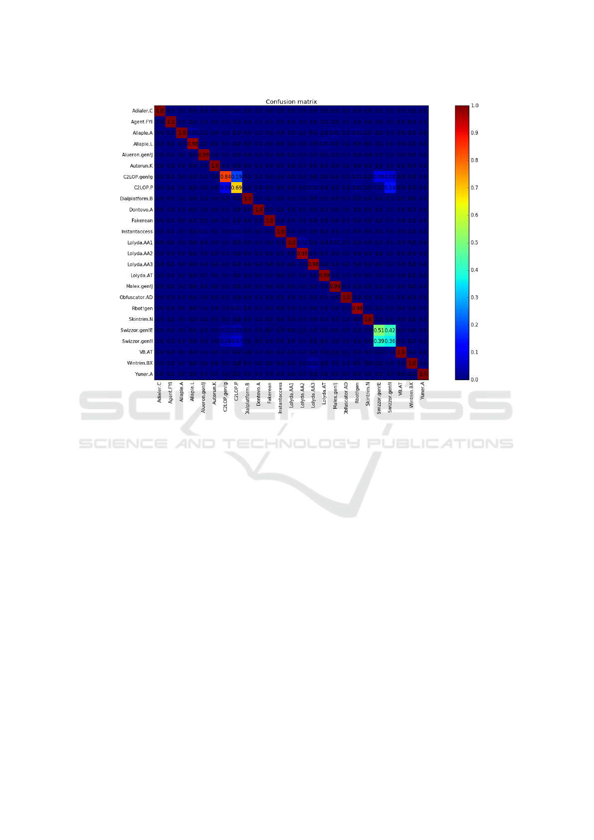
Figure 2: Confusion matrix for k-NN based on all features.

linear SVC, then eliminate the feature with the smal-

lest weight and recompute the linear SVC on this re-

duced feature set—this process is repeated until only

a single (strongest) feature remains. By retraining at

each step, we are able to account for the interactions

within the reduced feature set.

We found that when applying RFE to the Malicia

dataset, the full 320 gist features yielded the best re-

sults, but with about 60 features we are able to obtain

nearly optimal results. For this dataset, a graph of the

accuracy versus the number of features selected ap-

pears in Figure 5.

We also experimented with univariate feature se-

lection (UFS). In UFS, an SVC is constructed for

each individual feature and the resulting accuracies

are used to rank the features.

Applying UFS on the Malicia dataset, we ﬁnd that

with only the 60 highest ranked features, we can attain

an accuracy of almost 92%, which is within 1% of

that obtained with all 320 features. We conclude that

we can obtain near-optimal results using just 60 of

the 320 gist descriptors as features.

3.5 Robustness Experiments

Next, we consider attacks aimed at degrading the ef-

fectiveness of the gist-based score. First, we consider

experiments where we salt the malware samples with

spurious images. For this experiment, we test each of

the following three methods of salting images.

• Salt the samples of only one family with extrane-

ous images.

• Salt two closely related families with similar ex-

traneous images.

• Salt all families with the benign samples.

Intuitively, when only one family is salted with

an extraneous image we might expect that the over-

all classiﬁcation results will actually improve slightly.

This follows, because the samples in the salted family

should now be more distinct from other families—and

hence there will likely be fewer misclassiﬁcations in-

volving this particular family—while all other fami-

lies remain unchanged. To test this hypothesis, we

salted only the Allaple.L family of the Malimg data-

set. This resulted in the classiﬁcation accuracy for the

Allaple.L family improving from 98% to 100%.

Adialer.C

Agent.FYI

Allaple.A

Allaple.L

Alueron.gen!J

Autorun.K

C2LOP.gen!g

C2LOP.P

Dialplatform.B

Dontovo.A

Fakerean

Instantaccess

Lolyda.AA1

Lolyda.AA2

Lolyda.AA3

Lolyda.AT

Malex.gen!J

Obfuscator.AD

Rbot!gen

Skintrim.N

Swizzor.gen!E

Swizzor.gen!I

VB.AT

Wintrim.BX

Yuner.A

0.00

0.20

0.40

0.60

0.80

1.00

Precision

Recall

Figure 3: Precision and recall.

30 40

50 60

70 80 90

100

Training data percentage

Accuracy (percentage)

Figure 4: Accuracy vs training/testing split (Malicia data-

set).

For our next experiment, we salted two related fa-

milies with similar extraneous images. In this case,

we might intuitively expect that the accuracy will de-

crease for both of these families, as they are now more

similar to each other than they were before salting,

and this increased similarity will likely result in more

misclassiﬁcations. For this experiment, we chose the

Allaple.L and Allaple.A families and salted all sam-

ples in both families with images selected from an

external image dataset. We found that the classiﬁca-

tion accuracy for the Allaple.L and Allaple.A families

100

150

200

250

300

100

Number of features

Accuracy (percentage)

Figure 5: Accuracy vs number of features (RFE for Malicia

dataset).

both declined signiﬁcantly, as summarized in Table 4.

These results indicate that gist-based scoring is not

immune to this entirely straightforward obfuscation

attack. However, the decline in accuracy is relatively

modest, which shows that the gist-based score is so-

mewhat resilient, at least with respect to this simple

obfuscation strategy.

Next, we conducted an experiment where all mal-

ware samples were salted with benign executable ﬁ-

les. Similar techniques have previously been used

to defeat many statistical-based—and machine lear-

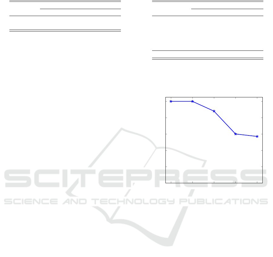
Table 4: Accuracy before and after salting.

Family

Accuracy

Before Salting After Salting

Allaple.A 100% 93%

Allaple.L 98% 85%

ning based—scores (Desai and Stamp, 2010; Lin and

Stamp, 2011; Singh et al., 2016). For this experiment,

we obtain an overall classiﬁcation accuracy of 92%,

which represents a signiﬁcant decline from the origi-

nal (unsalted) accuracy of 97%.

Finally, we test a slightly different salting strategy,

where the salting data is interleaved within the mal-

ware samples. Speciﬁcally, we interleaved selected

benign samples within the Allaple.A, Allaple.L, and

Fakerean families of the Malimg dataset. As in our

ﬁrst salting experiments, the results are slightly stron-

ger, with an accuracy of 93%.

Overall, these experimental results indicate that

gist-based scoring is reasonably robust against these

speciﬁc salting attacks. However, more research is

needed, and we remain conﬁdent that the there exists

a straightforward attack strategy that can be highly ef-

fective against gist-based scoring.

Next, we apply softmax regression and deep lear-

ning to the image-based malware classiﬁcation pro-

blem. In these experiments, we do not rely on gist

descriptors, but instead use only the raw bytes in the

image ﬁles as our feature. Our goal is to determine

whether techniques that require no preprocessing of

the data can be as successful as the gist-based score

considered above.

3.6 Softmax Regression

Logistic regression is a well-known algorithm that is

applicable to the binary classiﬁcation problem. Soft-

max regression is a generalization of logistic regres-

sion that can deal with multiple classes—the sigmoid

function from logistic regression is replaced by the

softmax function. A set of weights and biases must

be determined and these, along with the input data,

are used by the softmax function. The output consists

of probabilities for each class.

For our softmax experiments, we again use the

Malimg dataset. These experiments were performed

with n families, where n ranged from one to ﬁve. In

Table 5 we list families—for n = 1, we used only the

Adialer.C family, for n = 2 we used both Adialer.C

and Agent.FYI, and so on.

For these softmax experiments, as the number of

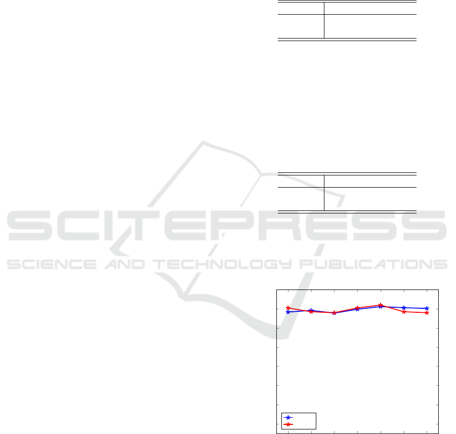
families increases, the classiﬁcation accuracy decre-

ases drastically—see Figure 6. These results are so-

mewhat surprising, with only 57% accuracy attained

Table 5: Number of samples per family.

Family

Number of samples

Training Testing Total

Adialer.C 100 22 122

Agent.FYI 98 18 116

Allaple.A 2655 294 2949

Allaple.L 1432 159 1591

Allueron.gen 179 19 198

Total 4464 512 4976

when ﬁve families were tested. We conclude that

for any signiﬁcant number of families, this softmax

classiﬁcation approach performs much worse than the

gist-based score considered above.

1 2 3 4

100

Number of families

Accuracy (percentage)

Figure 6: Softmax classiﬁcation accuracy.

3.7 Deep Learning Experiments

Deep learning using many layers of neural networks

is an increasingly popular technique in a wide variety

of challenging problem domains, including image re-

cognition and segmentation (Krizhevsky et al., 2012).

For example, Google’s Inceptionv3 and Facebook Ar-

tiﬁcial Intelligence Research (FAIR) have had good

success rates by applying deep learning to problems

in the ﬁelds of image classiﬁcation and object seg-

mentation, respectively (Szegedy et al., 2016; Pin-

heiro et al., 2015). In this section, we apply deep

learning to the malware classiﬁcation problem, trea-

ting malware binaries as images. We then compare

our deep learning results to the gist-based malware

classiﬁcation approach considered above.

3.8 TensorFlow for Deep Learning

Training a neural networks can be computationally in-

tensive. One of the reasons that neural networks have

gained popularity in recent years is due to advances

made in hardware and software that have rendered the

computational aspects of neural networks less daun-

ting (Oh and Jung, 2004). In particular, with recent

advances in GPU technology and software, it is now

practical to train neural networks on GPUs (Oh and

Jung, 2004; TensorFlow, 2017).

TensorFlow

is an open source software library

by Google that is designed for numerical computation

on data ﬂow graphs. TensorFlow is the successor of

the earlier closed source DistBelief (also from Goo-

gle) which was used for training and deploying neural

networks for pattern recognition (TensorFlow, 2017).

The unit of data in TensorFlow is a set of primi-

tive values in the form of an n-dimensional array. A

TensorFlow program builds a “computational graph,”

which is deﬁned as a series of TensorFlow operati-

ons arranged into a graph form. A node may or may

not have a tensor as its input but it usually produces a

tensor as output. Once the computational graph is cre-

ated, it can be evaluated by executing it, which con-

sists of creating a session to encapsulate the control

and state of the TensorFlow runtime, and executing

the graph within it (TensorFlow, 2017).

TensorFlow was used to conduct the deep lear-

ning experiments in this section. The model used

here relies on transfer learning, which involves star-

ting with a model pre-trained on another problem.

Then, we retrain this existing model on a similar pro-

blem. The motivation for this approach comes from

the fact that training deep learning model from scra-

tch is generally extremely computationally intensive,

while simply modifying an existing model can be or-

ders of magnitude faster, depending on the dataset.

For the experiments reported here, the model was

pre-trained on the ImageNet Large Visual Recogni-

tion Challenge dataset, and is capable of differenti-

ating between 1000 different image classes, such as

Dalmatian, helmet, motorcycle, person, etc. (Google

Codelabs, 2017). We then retrained this model on the

raw malware images in the Malimg dataset.

In addition to the software listed in Table 1, for

the deep learning experiments discussed here, we em-

ploy the TensorFlow architecture on an NVIDIA DI-

GITS DevBox provided by Ford Motor Company. All

experiments described in this section use 4 GPUs on

the NVIDIA DIGITS DevBox As previously mentio-

ned, the training and test data for these experiments is

form the Malimg dataset, which contains more than

9000 grayscale images representing malware from 25

malware families, as summarized in Table 2, above.

3.9 TensorFlow Results

As a ﬁrst experiment of our TensorFlow model, we

classiﬁed two very different families, Allaple.A and

Yuner.A, using a 90-10 split (i.e., 90% of images were

used for training and 10% for testing). When training,

we use 4000 iterations to retrain the model. These re-

sults are given in Table 6, and we note that all samples

were classiﬁed correctly.

Table 6: Accuracy results on Allaple.A and Yuner.A.

Images Accuracy

Training 3374 100%

Testing 375 100%

Next, as a more challenging test for our Ten-

sorFlow model, we classiﬁed two closely related fa-

milies, Allaple.A and Allaple.L, again using a 90-10

split and 4000 iterations to retrain the model. These

results are given in Table 7, and we again see that we

have achieved perfect classiﬁcation. These are cer-

tainly impressive initial results for this deep learning

approach.

Table 7: Accuracy results on Allaple.A and Allaple.L.

Images Accuracy

Training 4086 100%

Testing 454 100%

Finally, we attempt to classify samples from all 25

Malimg malware families. For these experiments, we

test various splits of the training and test data, ranging

from 30-70 to 90-10 split. The resulting accuracies

are given in Figure 7.

30 40

50 60

70 80 90

100

Training data percentage

Accuracy (percentage)

Testing

Training

Figure 7: Accuracy vs training/testing split for TensorFlow

experiments with all 25 Malimg families.

From the results in Figure 7, we see that by ap-

plying deep learning directly to raw image ﬁles, we

can attain a testing accuracy in excess of 98%, which

is as good as the accuracy obtained based on gist des-

criptors as reported in (Nataraj et al., 2011), and as

50 60

70 80 90

100

Training data percentage

Accuracy (percentage)

Testing

Training

Figure 8: Accuracy vs training/testing split for TensorFlow

experiments with all 25 Malimg families (balanced).

conﬁrmed by our results in Section 3.3, above.

As an aside, we note that according to Table 2,

the number of samples of the various malware types

in the Malimg dataset ranges from a high of 2949 for

the Allapple.A family to a low of just 80 for the Skin-

trim.N family. To determine a “balanced” accuracy,

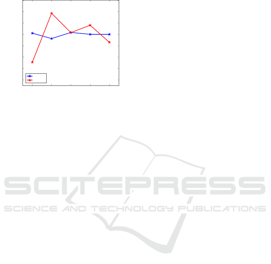
we repeated our deep learning experiments, using 80

samples from each family. The results of these expe-

riments are summarized here in Figure 8, where we

see the the testing accuracy is signiﬁcantly lower than

in the original unbalanced case. The large difference

between the unbalanced and balanced cases is most

likely due to the larger families being relatively easy

cases, as compared to the smaller families in the data-

set. This is worth noting since the unbalanced Malimg

dataset has been used in previous work (Nataraj et al.,

2011).

3.10 Discussion

One advantage of our deep learning strategy is that

it is likely to be much more efﬁcient than relying on

gist descriptors. While training a neural network from

scratch can be extremely costly, our re-training appro-

ach only required about 60ms per sample. We believe

this is competitive with virtually any machine lear-

ning technique. Furthermore, when training and sco-

ring via deep learning, there is no need to extract gist

descriptors for use as features—even with feature se-

lection, we still required at least 60 gist descriptors

to obtain near-optimal results. This savings in feature

extraction time is likely to give the deep learning ap-

proach a signiﬁcation advantage over the gist-based

score in actual practice.

4 CONCLUSION AND FUTURE

WORK

Our classiﬁcation experiments based on gist descrip-

tors conﬁrmed the results in (Nataraj et al., 2011) and

also showed that we could obtain equally strong re-

sults using only 60 gist features. In addition, we sho-

wed that the gist-based score is moderately robust in

the face of elementary obfuscations.

We conducted deep learning experiments that

yielded equally strong classiﬁcation results as the

gist-based experiments. Since there is no need to ex-

tract gist features, this deep learning technique is li-

kely to offer superior performance when scoring large

numbers of samples, as would be necessary when

using such techniques in practice. For future work,

we plan to accurately quantify the efﬁciency advan-

tage of our deep learning approach, as compared to

techniques that rely on gist descriptors.

Additional future work will include more substan-

tial robustness testing. The gist-based score appears

to be somewhat robust, but to date, our experiments

along these lines have been limited and inconclusive.

A careful and detailed analysis of the robustness of

the gist-based score—as compared to our deep lear-

ning score—would be useful. At the least such an

analysis will help to focus future research in directi-

ons that are most likely to yield improvements over

the existing state of the art.

ACKNOWLEDGEMENTS

We would like to thank Ford Motor Company for ge-

nerously allowing us to use their hardware and pre-

trained models for the deep learning experiments re-

ported here.

REFERENCES

Bayer, U., Moser, A., Kruegel, C., and Kirda, E. (2006).

Dynamic analysis of malicious code. Journal in Com-

puter Virology, 2(1):67–77.

Desai, P. and Stamp, M. (2010). A highly metamorphic

virus generator. International Journal of Multimedia

Intelligence and Security, 1(4):402–427.

Douze, M., J

egou, H., Sandhawalia, H., Amsaleg, L., and

Schmid, C. (2009). Evaluation of gist descriptors for

web-scale image search. In Proceedings of the ACM

International Conference on Image and Video Retrie-

val, CIVR ’09, pages 19:1–19:8, New York, NY, USA.

ACM.

Google Codelabs (2017). Tensorﬂow for poets. https://

codelabs.developers.google.com/codelabs/tensorﬂow-

for-poets/.

Krizhevsky, A., Sutskever, I., and Hinton, G. E. (2012).

Imagenet classiﬁcation with deep convolutional neu-

ral networks. In Advances in Neural Information Pro-

cessing Systems, pages 1097–1105.

Lin, D. and Stamp, M. (2011). Hunting for undetectable

metamorphic viruses. Journal in Computer Virology,

7(3):201–214.

Moser, A., Kruegel, C., and Kirda, E. (2007). Limits of

static analysis for malware detection. In Twenty-Third

Annual Computer Security Applications Conference,

ACSAC 2007.

Nappa, A., Raﬁque, M. Z., and Caballero, J. (2015). The

malicia dataset: Identiﬁcation and analysis of drive-by

download operations. International Journal of Infor-

mation Security, 14(1):15–33.

Nataraj, L., Karthikeyan, S., Jacob, G., and Manjunath,

B. S. (2011). Malware images: Visualization and au-

tomatic classiﬁcation. In Proceedings of the 8th Inter-

national Symposium on Visualization for Cyber Secu-

rity, VizSec ’11, pages 4:1–4:7, New York, NY, USA.

ACM.

Oh, K.-S. and Jung, K. (2004). GPU implementation of

neural networks. Pattern Recognition, 37(6):1311–

1314.

Oliva, A. and Torralba, A. (2001). Modeling the shape

of the scene: A holistic representation of the spatial

envelope. International Journal of Computer Vision,

42(3):145–175.

Pinheiro, P. O., Collobert, R., and Dollar, P. (2015). Le-

arning to segment object candidates. In Advances in

Neural Information Processing Systems, pages 1990–

1998.

Selvin, V. R. S. (2017). Malware scores based on image

processing. Master’s Project, Department of Compu-

ter Science, San Jose State University.

Sharif, M. I., Lanzi, A., Gifﬁn, J. T., and Lee, W. (2008).

Impeding malware analysis using conditional code

obfuscation. In Proceedings of the Network and Dis-

tributed System Security Symposium, NDSS 2008.

Singh, T., Troia, F. D., Visaggio, C. A., Austin, T. H., and

Stamp, M. (2016). Support vector machines and mal-

ware detection. Journal of Computer Virology and

Hacking Techniques, 12(4):203–212.

Szegedy, C., Vanhoucke, V., Ioffe, S., Shlens, J., and Wo-

jna, Z. (2016). Rethinking the inception architecture

for computer vision. In Proceedings of the IEEE Con-

ference on Computer Vision and Pattern Recognition,

CVPR 2016, pages 2818–2826.

TensorFlow (2017). Getting started with tensorﬂow.

https://www.tensorﬂow.org/get started/get started.

Accessed 2017-04-22.

You, I. and Yim, K. (2010). Malware obfuscation techni-

ques: A brief survey. In 2010 International Confe-

rence on Broadband, Wireless Computing, Commu-

nication and Applications, BWCCA ’10, pages 297–

300.