An Efficiency Frontier based Model for Cloud Computing Provider
Selection and Ranking
Lucas Borges de Moraes
1
, Pedro Cirne
2
, Fernando Matos
3
, Rafael Stubs Parpinelli
1
and Adriano Fiorese
1
1
Dept. of Computer Science (DCC), Santa Catarina State University (UDESC), Joinville, Brazil
2
Instituto de Telecomunicac¸
˜
oes, Aveiro, Portugal
3
Dept. of Computer Systems (DSC), Federal University of Para
´
ıba (UFPB), Jo
˜
ao Pessoa, Brazil
Keywords:
Cloud Computing Provider, Data Envelopment Analysis, Performance Indicator, Selection Method, Ranking.
Abstract:
Cloud computing become a successful service model that allows hosting and distribution of computational re-
sources all around the world, via Internet and on demand. This success leveraged and popularized its adoption
into all major IT companies. Based on this success, a large number of new companies were competitively
created as providers of cloud computing services. This fact can difficult the customer ability to choose among
those several cloud providers the most appropriate one to attend their requirements and computing needs.
Therefore, this work aims to propose a model capable of selecting and ranking cloud providers according the
analysis on the most efficient ones using a popular Multicriteria Decision Analysis (MCDA) method called
Data Envelopment Analysis (DEA), that calculates efficiency using Linear Programming (LP) techniques. To
accomplish that, the efficiency modeling is based on the analysis of each Performance Indicator (PI) values
desired by the customer and the available ones in the cloud provider database. An example of the method’s
usage is given to illustrate the model operation, selection results and final provider ranking for five hypothetical
customer requests and for ten providers.
1 INTRODUCTION
The modernization of society brought the need of
efficient, affordable and on-demand computational
resources. The evolution of telecommunications
technology, especially computer networks, provided
an environment that leveraged the rise of cloud
computing paradigm. Cloud computing has shown
a new vision of service delivery to its customers. It
became a differentiated service model of facilitated
hosting and distribution of computer services all over
the world via Internet.
Cloud computing abstracts to the customer its
complex internal infrastructure and architecture keep
by the service provider (Hogan et al., 2013). Thus, to
use the service, the customer don’t need to perform
installations, configurations, software updates or
purchase specialized hardware (Zhang et al., 2010).
That is, all computational resources that the customer
needs, can be managed and made available by the
cloud provider. On this way, the cloud computing
paradigm has brought the benefit of better use of
computational resources, saving hardware, energy
and time. In addition to being a convenient service,
it is easily accessible via the network and it is only
charged for the time that is used (Hogan et al., 2013).
The success of cloud computing paradigm is
noticeable and it has been adopted in major IT
companies like Google, Amazon, Microsoft, IBM,
and Salesforce.com and has become a good source
of development and investment for both academy and
industry (Zhou et al., 2010). This success leveraged
the rising of a large number of new companies
as cloud computing infrastructure providers. But,
the demand for quality also increased. With the
increasing amount of new cloud providers the task
of choosing and selecting which cloud providers
are the most suitable for each customer’s needs
has become a complex process. The process of
measuring the quality of each provider and compare
them is not trivial, as there are usually many factors
involved, many criteria to be studied and checked out
throughout the process. Cloud providers should be
able to measure their service provided (an essential
characteristic called “Measured service”) (Hogan
et al., 2013) and publicly share such information, in
Borges de Moraes, L., Cirne, P., Matos, F., Stubs Parpinelli, R. and Fiorese, A.
An Efficiency Frontier based Model for Cloud Computing Provider Selection and Ranking.
DOI: 10.5220/0006775705430554
In Proceedings of the 20th International Conference on Enter prise Information Systems (ICEIS 2018), pages 543-554
ISBN: 978-989-758-298-1
Copyright
c
 2019 by SCITEPRESS – Science and Technology Publications, Lda. All rights reserved
543

the form of criteria or PIs, for example.The quality
measure of a cloud provider can be done by the
numerical and systematical measure of quality of each
provider’s Performance Indicators (PIs), reaching a
certain score. Thus, providers can be ranked and the
provider that offer the higher score is theoretically the
most appropriate provider to that customer.
PIs are tools that enable a systematic summarized
information collection about a particular aspect of
an organization. They are metrics responsible for
quantifying (assigning a value) the objects of study to
be measured, allowing organizations to monitor and
control their own performance over time. PIs should
be carefully measured in periods of regular time
so that they are representative to the characteristic
they represent. Example of some PIs found in
the literature: Computer resources offered, cost of
service, supported operating systems, security level,
response time, availability, recoverability, accuracy,
reliability, transparency, usability, customer support,
etc. (Garg et al., 2013)(Baranwal and Vidyarthi,
2014). PIs are classified into quantitative discrete or
quantitative continuous, i.e., they can be expressed
numerically and worked algebraically; and qualitative
ordered or qualitative unordered, i.e., they have
distinct states, levels or categories defined by an
exhaustive and mutually exclusive set of sub classes,
which may be ordered (possesses a logical gradation
among its sub classes, giving idea of a progression) or
not (Jain, 1991).
It is also possible to classify qualitative PIs
according to the behavior of their utility function, i.e.,
how useful the PI becomes when its numerical value
varies (Jain, 1991):
• HB: Higher is Better. The highest possible values
for this indicator are preferred, e.g., amount of
memory, availability, etc.
• LB: Lower is Better. The smallest possible values
for this indicator are preferred, e.g., cost, delay,
latency, etc.
• NB: Nominal is Best. A particular value is
considered to be the best, higher and lower values
are undesirable, e.g., total system utilization.
Cloud computing has a noticeable set of PIs
organized in a hierarchical framework divided into
seven major categories (accountability, agility, service
assurance, financial, performance, security and
privacy, usability), called Service Measurement Index
(SMI), developed by Cloud Service Measurement
Index Consortium (CSMIC) (CSMIC, 2014).
This framework provide a standardized model for
measuring and comparing the quality of cloud
computing services, identifying and explaining
metrics that can be used by cloud computing
consumers. SMI has been used as the basis for
several works as: (Garg et al., 2013; Baranwal and
Vidyarthi, 2014; Achar and Thilagam, 2014; Wagle
et al., 2015; Shirur and Swamy, 2015).
The Data Envelopment Analysis (DEA) is a
well-known method for decision-making support,
introduced first by Charnes at al. in 1978 (Charnes
et al., 1978). DEA belogs to the called Multicriteria
Decision Analysis (MCDA) (Ishizaka and Nemery,
2013) area. According to it, each solution alternative
is called DMU (Decision Making Unit) and each
criterion is an input or an output. DEA selects
DMUs calculating the efficiency of each one. The
efficiency is defined as the ratio of the sum of
its weighted outputs to the sum of its weighted
inputs (Ramanathan, 2003). So, outputs are criteria to
be maximized and inputs as criteria to be minimized
for better efficiency. DEA modeling transform
this definition into a set of equations of Linear
Programming (LP) to be solved for a LP algorithmic
(e.g., Simplex). What distinguishes DEA is that
the weights assigned to outputs and inputs are not
allocated by its users, but automatically chosen
by the method, so that do the most benefit to
each DMU (Ramanathan, 2003). DMUs with max
efficiency (value 1, which means 100%) form a set
called efficiency frontier. DEA have two main models
(CCR and BCC) that consider or not if any variation
in the inputs produces a proportional variation in the
outputs, and two orientations, i.e., inputs or outputs,
that define if the method will try minimize inputs or
maximize outputs, respectively.
Thus, the purpose of this work is to present a
new model of cloud computing selection and ranking
that uses the DEA method, where the cloud providers
efficiency is analyzed using the consumer requested
PIs values (that specifies their computational needs)
and the cloud provider PIs values, to choose the
best provider to the consumer request. The main
contribution of this paper is the DEA input and
output variables modeling and equations proposal
based on the aggregation and transformation of PIs
(PIs conversion to DEA inputs and outputs variables),
applied to the problem of selecting cloud computing
providers.
The remainder of this paper is organized as
follows: Section 2 presents related works to the
selection, scoring and ranking of cloud providers
based on MCDA methods. Section 3 explains how
the problem of selecting cloud providers is modelled,
its scope and main elements (provider database and
customer request). Section 4 presents the proposed
model using DEA, that selects and ranks different
ICEIS 2018 - 20th International Conference on Enterprise Information Systems
544

cloud providers based on their PIs and customer’s
interest PIs (requested PIs). Section 5 illustrates an
example, with hypothetical data, that represents an
application of the proposed model, in order to validate
it and to demonstrate its operation the results. Finally,
Section 6 presents the final considerations.
2 RELATED WORKS
Selecting the most appropriate cloud provider is a
problem that has taken a lot of attention in scientific
works in recent decade due the significant growth
in the numbers of providers. The problem is cited
several times and addressed in different ways. This
section presents some papers related to the problem
of selecting and ranking cloud services or providers,
especially using multiple MCDA methods (AHP,
ANP, TOPSIS, fuzzy TOPSIS, DEA, etc.) (Ishizaka
and Nemery, 2013).
CloudCmp (Li et al., 2010) is the first systematic
comparator found for performance and cost of public
cloud providers. This tool is developed to guide
customers in selecting the best cost-effective provider
for their applications through the use of benchmarks.
It can measure features such as elastic computing,
persistent storage and the networking services offered
of four cloud servers: Amazon AWS, Microsoft
Azure, Google AppEngine and Rackspace. This
study was a start about the concern of the problem
of choosing the best cloud provider, although direct
measurement of QoS metrics by benchmarks can be
problematic, unstable and is currently underused.
A brokerage approach using an indexing
technique is used to create and index distinct cloud
services to assist the selection of cloud providers to
users (Sundareswaran et al., 2012). The brokers are
responsible for selecting the appropriate service for
each client and have a contract with the providers,
collecting their properties (PIs), and with the
consumers, collecting their service requirements.
Brokers analyze and index service providers
according to the similarity of their properties. Each
property (except service type) has a unique encoding,
associated with each discrete ranges of possible
values that it can assume. Upon receiving a selection
request, the broker will search the index to identify
an orderly list of candidate providers based on how
well they match the needs of the users. The generated
index key is formed by the concatenation of the
encoding type of service offered by the provider
with a “Xor” operator among all the other encoded
properties offered by such provider. The providers
are indexed in a tree structure called “B+-tree”.
The approach is tested with a data set with six
real providers (Amazon EC2, Windows Azure,
Rackspace, Salesforce, Joynet, Google Clouds) and
nine PIs (service type, security level, QoS level,
measurement unit, pricing unit, instance sizes,
operating system, pricing and location-based prices).
The framework called
“SMICloud” (Garg et al., 2013) can rank cloud
computing services using the indicators of the
SMI (CSMIC, 2014). The framework measures
the QoS of each cloud provider and ranks them
based on this calculated quality. For this, it uses
the Analytical Hierarchical Process (AHP) method
(Saaty, 1990) for the calculation of the quality of the
providers. Each indicator (AHP attribute/criteria)
can be essential or non-essential and can be boolean,
numeric, unordered set or range type. A small study
case is provided at the end with three real provider:
Amazon EC2, Windows Azure and Rackspace. The
main SMI attributes used are accountability level,
agility (capacity and elasticity time), assurance
(availability, stability, serviceability), cost (VM,
storage), performance (response time) and security
level. The unavailable data such as the security
level are randomly assigned to each provider. The
method is appropriate and logically plausible,
although it seems that the assembly of the hierarchy
for a large number of providers and PIs seems to
be complex and tiresome. This method may also
not be appropriate to treat qualitative PIs such as
accountability and security levels. It also has implicit
the subjectivity problem of the arbitrary choice of
AHP weights (Whaiduzzaman et al., 2014).
The ranked voting model proposed by Baranwal
and Vidyarthi (Baranwal and Vidyarthi, 2014) can
rank and select cloud services based on users QoS
expectation metrics. The base QoS metrics are the
SMI ones. The main actors of the model are the
cloud exchange, cloud coordinator and cloud broker
with a data directory that contains all information
about providers which are required in selection of the
best one. The metrics are divide in to two categories:
application dependent and user dependent. Values
of metrics can be of different types like numeric,
boolean, range type, unordered set and data centre
value. In ranked voting system, each metric will
act as a voter, and cloud providers are candidates
for them. The method proposed to analyze ranked
voting data was DEA (Cook and Kress, 1990).
A very similar proposal to this model is
the measure index framework for cloud
service (Shirur and Swamy, 2015), with the same
QoS metrics (SMI) and same ranked voting method.
The main actors of the framework are cloud
An Efficiency Frontier based Model for Cloud Computing Provider Selection and Ranking
545

swapping, cloud coordinator, cloud user and cloud
mediate. The cloud index contains all information
about service providers which are required in
selection of a best provider. The description of each
module or phase needs a better explanation and
practical examples for better understanding of the
method are also needed.
A brokerage approach developed by Achar and
Thilagam (Achar and Thilagam, 2014) can rank IaaS
cloud providers using a broker measuring the QoS
of each provider, prioritizing those most appropriate
to the needs of each request to the broker. The key
elements of the approach are: the broker, the requester
of a cloud provider (consumer), and a list with “n”
cloud providers. The selection involves three steps:
Identify which criteria are appropriate to the request
by identifying the necessary PIs present in the SMI;
access the weight of each of these criteria using the
AHP method; and rank each provider using TOPSIS
(Technique for Order Preference by Similarity to
Ideal Solution) (Hwang and Yoon, 1981). TOPSIS is
used to select the alternative that is closest to the ideal
solution and further away from the ideal negative
solution. The final example have six hypothetical
providers with four PIs (availability, accountability,
cost and security). The use of TOPSIS appears
to be promising, but more analysis and examples
are need for further conclusions, with real data and
users requests. Qualitative PIs need an appropriate
modeling too.
The evaluation model proposed by Wagle et
al. (Wagle et al., 2015) verifies quality and status of
cloud services by an ordered heat map checking the
commit of the Service Level Agreements (SLA). The
data is obtained by cloud auditors and is viewed
via a heat map ordered by the performance of
each provider, showing them in descending order
of overall QoS provided. This map represents a
visual recommendation and aid system for cloud
users and brokers. The main metrics are again
based on the SMI and are: availability (divided
in up-time, downtime and interruption frequency),
reliability (load balancing, MTBF, recoverability),
performance (latency, response time and throughput),
cost (snapshot and storage cost) and security
(authentication, encryption, and auditing). This
selection approach is visual and apparently does not
rely with an automated method for a final decision of
which provider should be selected, making it complex
to work if the number providers and QoS metrics
grows.
Techniques of MCDA are continuously modeled
to select cloud providers, e.g., TOPSIS and Fuzzy
TOPSIS (Sodhi and T V, 2012), with the conjugated
use with AHP and ANP (Jaiswal and Mishra, 2017).
The purpose is to use TOPSIS and fuzzy TOPSIS to
identify the most effective cloud service according
users’ requirement. To evaluate criteria weights for
each of these methods the AHP or ANP methods are
used and the results are compared at the end. For
performance evaluation is used an example with four
hypothetical providers with data gathered from cloud-
harmony.com and with eight arbitrary quantitative
criteria. The presented examples are confusing,
subjective and dependent on the weights assigned by
the user, making the proposed method’s efficiency
questionable for large quantities of providers. The
method does not seem to be able to handle subjective
criteria.
The matching method proposed by Moraes
et al. (Moraes et al., 2017) is a deterministic
logical/mathematical algorithm that can score and
rank an extensive list of cloud providers based on the
value, type (quantitative or qualitative), nature (HB,
LB, NB) and importance (essential or non-essential)
of each PI requested by the customer. The method is
agnostic and generic to what PIs are used (whether
quantitative or qualitative) and can handle tolerances
specified for each PI. The algorithm is able to rank
providers that are the most suitable for each different
request. The score is calculated for each provider
individually and varies in the range of 0 to 1. The
closer to 1 the more adequate is that provider to
satisfy the request. The method is divided into
three stages (Elimination of incompatible providers,
scoring quantitative and/or qualitative PIs by level
of importance and calculation of final score per
provider). It returns a list with the highest-ranked
providers, containing their name, the total score and
their percentage of how many PIs of the request
has been attended. A simple example is given
with five hypothetical providers and seven different
PIs. Although this method handles quantitative and
qualitative PIs, it does not assess efficiency regarding
the matched cloud providers.
3 MODELING THE PROBLEM OF
SELECTING CLOUD
PROVIDERS
Given a finite initial non-empty set P with n different
cloud computing providers, each provider with M
distinct associated (PIs), the problem is to choose
the best subset of providers P
0
⊂ P, in order to
maximize the attendance of a specific request from
cloud consumers with the least possible amount
ICEIS 2018 - 20th International Conference on Enterprise Information Systems
546

of providers and resources and with the lowest
cost involved. The consumer request represents its
computing needs to achieve its goals and must inform
all the m PIs of interest, which must be a subset
of the provider’s associated PIs, with the respective
desirable value (X
j
). Other features can be informed
in request, such as the importance weight of each PIs
of interest (w
j
), the tolerance value of the desirable
one (t
j
) and even force the type of behavior of
the PI (Higher is Better or HB, Lower is Better,
Nominal is Best or NB) (Jain, 1991) – Assuming
the user knows what he’s doing. In practice,
a third-party (e.g., the server where the selection
method is hosted) must have an extensive database
containing a list of cloud computing providers. Each
provider has a respective set of PIs, fed directly or
indirectly by organizations such as brokers and/or
cloud auditors (Hogan et al., 2013) or maintained by
the cloud providers themselves in order to create a
conjugated database. Table 1 presents an example of a
possible database, agnostic and generic for all kind of
providers and quantitative PIs. The existence of this
database is an essential requirement for the model,
with the registered PIs and their types and values.
Table 1: Example of a generic cloud providers database.
Name Type P
1
P
2
P
3
... P
n
PI
1
HB/LB/NB x
11
x
21
x
31
... x
n1
PI
2
HB/LB/NB x
12
x
22
x
32
... x
n2
PI
3
HB/LB/NB x
13
x
23
x
33
... x
n3
... ... ... ... ... ... ...
PI
M
HB/LB/NB x
1M
x
2M
x
3M
... x
nM
Cost LB y
1
y
2
y
3
... y
n
A notably relevant PI used for selecting cloud
providers is cost. Cost is a PI to be always considered,
even if it is not informed by the customer in the
request, since it is a value that is always desirable
to minimize (LB). Table 2 shows a generic customer
(cloud computing service consumer) request, with all
fields that can be informed to the selection method.
Important to mention that PI name (identifier, unique)
and desired value are mandatory information, the
other are optional.
Table 2: Generic customer request.
Name Type Value Tolerance Weight
PI
1
. X
1
t
1
w
1
PI
2
NB X
2
t
2
w
2
PI
3
. X
3
t
3
w
3
... ... ... ... ...
PI
m
. X
m
t
m
w
m
Request column Type forces the PI type
overwriting the default type specified in the cloud
providers PI’s database (e.g., PI
2
will be NB).
In practical terms, it is informed after PI name,
between brackets (“[” and “]”). The default PI’s
value tolerance is zero, but it can be changed if it is
informed after the desired value with a positive real
(or integer) number between brackets. The default
weight of each PI is 1, but can be changed too, by
the customer. The PI Cost shouldn’t be added in the
request explicitly, since it will be used as an exclusive
DEA input called “Costs” because of its importance.
PI Cost is always LB, which means it can’t be forced
to be another type.
4 THE PROPOSED MODEL
This section aims to present and discuss the proposed
cloud service providers selection model. Figure 1
presents the proposed model for selecting and
ranking cloud provider based on its PIs using
DEA method. Each provider, can measure and
store their set of PIs, or contract an external
cloud agent such as Cloud Auditor or Cloud
Broker (Hogan et al., 2013) and passing this data
to a cooperative and publicly accessible database.
A total of m PIs of interest should be chosen by
the customer according to its goals towards cloud
providers. The customer will have a support and
informative interface, informing the available PIs
and able to collect the selected one’s weight. The
database of cloud provider candidates and their
PIs can be fed indirectly through websites such
as “Cloud Harmony” (https://cloudharmony.com)
and “Cloudorado” (http://www.cloudorado.com/) or
through cloud providers by their own (e.g: Amazon,
Microsoft) or it can be consolidated by third parties.
The database and the request must be first
properly converted to a format that DEA can work to
calculate the efficiency of each provider, generating
an efficiency frontier. This efficiency frontier frames
the set of providers that compared with others are
100% efficient, so any provider outside this frontier
will have a lower value of efficiency. Thus, in order to
feed the DEA method with the appropriate input and
output variables need to make a paired comparison
comprising efficiency among the cloud providers
candidates, a PIs converter is need in order to
compose these variables. Therefore, in this case, each
cloud provider is considered a Decision Making Unit
(DMU) of DEA, each one with two input variables
called “Resources” (“Res.”) and “Costs” (“Cost.”)
and two output variables called “Suitability”(“Suit.”)
and “Leftovers” (“Left.”). The set of providers
selected by DEA can be ranked using a simple
logical routine, using the converted/calculated input
An Efficiency Frontier based Model for Cloud Computing Provider Selection and Ranking
547

(...)
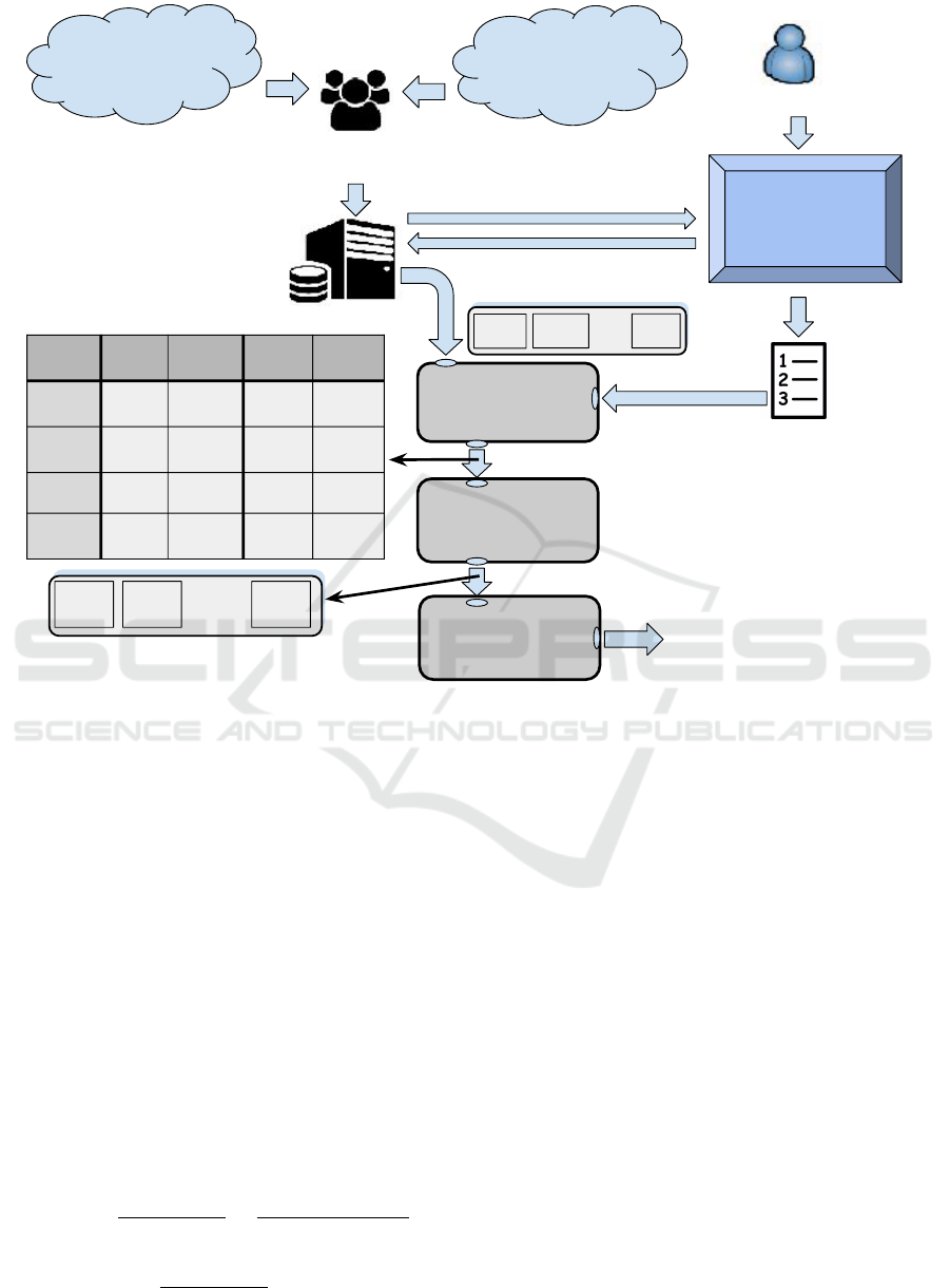
Cloud
Provider 1
Cloud
Provider n
Cloud Providers
Database
Customer
Customer
Interface
Customer
Request
DEA Input
Converter
DEA
Method
Efficiency Frontier
P’ with n’ elements
DMU Res. Cost. Suit. Left.
P1 A1 B1 C1 D1
P2 A2 B2 C2 D2
(...) (...) (...) (...) (...)
Pn An Bn Cn Dn
Ranking
Routine
P1 P3
Pn’
(...)
Rank Prov. Stat.
1 P3 Info1
2 Pn’ Info2
(…) (...)
n’ P1 Info n’
Third Party
Cloud Broker/Auditor
P1
P2
Pn
(...)
Initial Provider List
Figure 1: Proposed model to select and rank cloud providers using DEA.
and output variable by DEA input converter. The
following subsections expose the model steps and
mechanisms for calculating the score and ranking
each cloud provider.
4.1 DEA Input and Output Converter
Identify which inputs and outputs DEA have to
use for calculating efficiency is an essential step
for the correct use of this MCDA method. Each
DMU, i.e., each cloud provider has a constant
pre-defined number of inputs and outputs. The
efficiency in DEA, is defined as the ratio of the sum
of its weighted outputs to the sum of its weighted
inputs (Ramanathan, 2003; Ishizaka and Nemery,
2013), as shown in Equation 1, which is subject to
the constraint modeled in Equation 2.
E f f
DMU
=
Out puts
DMU
Inputs
DMU
=
∑
s
k=1
u
k
∗ O
k(DMU)
∑
r
l=1
v
l
∗ I
l(DMU)
(1)
0 ≤
∑
s
k=1
u
k
∗ O
ki
∑
r
l=1
v
l
∗ I
li
≤ 1,∀i (2)
It is important to note that u
k
,v
l
≥ 0, ∀k,l;
i = DMU
1
,DMU
2
,...,DMU
n
; k = 1,2,..., s and l =
1,2,...,r; where s is the total amount of outputs and r
the total amount of inputs; u
k
is the weight associated
with each output and v
l
the weight associated with
each input. So, the DMU that produces more outputs
with less inputs that the others will be evaluated
with better efficiency values. The weights assigned
to outputs (u
k
) and inputs (v
l
) are not allocated by
users (Ramanathan, 2003). Moreover, they do not
rely on a common set of weights for all providers.
Instead, a different set of weights is calculated by
a linear optimization procedure in order to allow
providers to produce the best results possible. The
set of DMUs with efficiency of 1 (means 100%) form
DEA’s efficiency frontier. Therefore, regarding the
problem addressed using DEA, each cloud provider
has two inputs and two outputs identified:
• Inputs (criteria to be minimized):
1. Resources: Corresponds to the weighted
average of the normalized values present in
the provider database. The used weights
are the PI’s weight present in the consumer
ICEIS 2018 - 20th International Conference on Enterprise Information Systems
548

request. Resources are basically inversely
proportional to the sum of all the gross
resources (represented by each PI) of each
provider. Its calculation is directly influenced
by PI’s type (HB, LB or NB).
2. Costs: Corresponds to the ratio of the provider
cost divided by the cost of the most expensive
provider in database.
• Outputs (criteria to be maximized):
1. Suitability: Is the weighted average (weighted
by each PI weight in the request) of the
attending (Equation 3) condition of each
provider’s PI, according to the customer request
(except cost). Basically, it indicates how
appropriate the provider is to the request.
2. Leftovers: Is the weighted average (weighted
by each HB and LB PI weight in the request) of
all the resources that had left in the provider,
after attending the request (for HB and LB,
only). That is, if the provider offers more
resources than the request asks for.
All these inputs and outputs are normalized
between 0 and 1. Equation 3 presents the PI
attendance condition, i.e., whether the requested PI’s
values can be satisfied by the cloud provider. It
takes into account the type of each PI (HB, LB or
NB), its value (the cloud provider value x
i j
present
in the database and the consumer desired value X
j
)
and tolerance value that is optional and should be
specified in the request, otherwise, it will be zero.
Attend(PI
j
,x
i j
,X
j
,t
j
) =







x
i j
≥ (X
j
−t
j
), if PI
j
∈ HB
x
i j
≤ (X
j
+t
j
), if PI
j
∈ LB
x
i j
≥ (X
j
−t
j
) and
x
i j
≤ (X
j
+t
j
), if PI
j
∈ NB
(3)
Where i = 1, 2,3,..., n (total number of providers);
j = 1,2,3, ...,m (total number of PIs in customer
request).
Moreover, in order to convert PI’s values it is
necessary to take into consideration the normalization
aspect. To accomplish that, formulation used take
into consideration maximum or minimum value of a
particular PI comprising all the cloud providers being
analyzed. Thus, let be PI
n
j
= {x
1 j
,x
2 j
,...,x
n j
} the set
of values corresponding to the PI
j
of all the n cloud
providers available. Equations 4 and 5 show how the
inputs “Resources” and “Costs” are converted for
the provider P
i
, respectively, and Equations 6 and 7
calculate the outputs “Suitability” and “Leftovers”,
respectively.
Di f = Max(PI
n
j
,X
j
) − Min(PI
n
j
,X
j
)
R =
m
∑
j=1
w
j
∗















1 −
x
i j
Max(PI
n
j
)
, if PI
j
∈ HB
x
i j
Max(PI
n
j
)
, if PI
j
∈ LB
|x
i j
− X
j
|
Di f
, if PI
j
∈ NB
Res(P
i
) =
R
∑
m
j=1
w
j
!
α
(4)
Costs(P
i
) =

y
i
Max(y
1
,y
2
,...,y
n
)

β
(5)
Suit(P
i
) =
∑
m
j=1
w
j
∗ Attend(PI
j
,x
i j
,X
j
,t
j
)
∑
m
j=1
w
j
!
γ
(6)
L =
m
HB
+m
LB
∑
j=1
w
j
∗













x
i j
− X
j
Max(PI
n
j
) − X
j
, if condition
1
1 −
x
i j
− X
j
Max(PI
n
j
) − X
j
, if condition
2
0 , otherwise
Le f t(P
i
) =






L
m
HB
+m
LB
∑
j=1
w
j






δ
(7)
It is important to note that i = 1,2,..., n; j =
1,2,...,m; α,β,γ, δ = 1, 2,3,...; m
HB
,m
LB
,m
NB
=
0,1,2,..., subject to m
HB
+ m
LB
+ m
NB
= m; where
Di f is the difference between the maximum value
of a particular NB PI
j
value and the user requested
PI
j
value (X
j
) and the minimum value of the
same. In other words, Di f is the maximum possible
distance (diference) between all the values of that
NB PI
j
, and that desired one in the request (X
j
).
Also, it is important to note that condition
1
=
Attend(PI
j
,x
i j
,X
j
,0) and PI
j
∈ HB; condition
2
=
Attend(PI
j
,x
i j
,X
j
,0) and PI
j
∈ LB. In addition, in
case X
j
≥ Max(PI
n
j
) happens, then, the “Leftovers”
value for that PI
j
is always zero ∀P
i
,x
i j
. The variable
factors α,β, γ,δ are responsible for transforming all
the inputs/outputs “Resources”, “Costs”, “Suitability”
and “Leftovers”, respectively, into functions with
a variation (increase/decrease), e.g., linear (1) is
default, quadratic (2), cubic (3), etc. That is, the
higher the value of such factors, the more significantly
numerically these inputs/outputs will be affected for
each change made. The higher the factor, the greater
the loss of punctuation for every provider that does
An Efficiency Frontier based Model for Cloud Computing Provider Selection and Ranking
549

not reach 1 (efficient), since the numbers are always
between 0 and 1. The farther from 1 and closer
to 0, the more score the provider will lose. For
more critical input/output, it is appropriate increase its
associated factor. Bearing this in mind, the considered
most critical feature is “Suitability”. Therefore, its
factor will be 2 (γ = 2), and for the others they will be
1 (linear variation).
4.2 An Efficient Way to Calculate PIs
Weights
As can be noticed, the conversion of PI values into
DEA input variable “Resources” and output variables
“Suitability” and “Leftovers” depends on the w
j
PI
weights, according Equations 4; 6; 7, respectively.
These weights are the user responsibility. However,
assigning weights for each PI is not necessarily a
trivial task, much more if there are so many involved.
An efficient technique for calculating, instead of
arbitrarily assigning, each PI weight is using a matrix
of judgments (Moraes et al., 2017). A judgment
matrix aims to model relationships (e.g.: importance,
necessity, discrepancy, value, etc.) between the
judged elements (Saaty, 2004). In this case, the
elements to be judged (regarding the determination of
weights) are the PI importance weights. Therefore,
in this case the customer provides how important
a PI is regarding the others, instead of a weight
value. Thus, the judgment matrix is a matrix with
dimension n, wherein each row and each column
represents a different PI. This technique is used
several times in the decision-making method called
Analytic Hierarchy Process (AHP) (Saaty, 2004).
Table 3 presents a possible example of judgment
matrix with four different non-cost PIs (cost doesn’t
need to have its importance/weight calculated,
according our proposed convertion model). The
assigned values are based on the scale of Saaty (Saaty,
2004). In this case, the values in the judgment matrix
indicate how important is the line element i with
respect to the column element j. That is, PI
1
is
two times more important that PI
2
; four times more
important that PI
3
and eight times more important that
PI
4
. Moreover, PI
2
is two times more important that
PI
3
and four times more important that PI
4
. On its
turn, PI
3
is three times more important that PI
4
. Thus,
following this methodology to build the judgment
matrix, it is obtained all values in the diagonal equal
to 1 and the observed inversions. On the last line, the
elements of each column are summed up in order to
advance the next step to find the weights, which is the
normalization of this matrix. Following, the matrix
normalization takes place. This process takes each
column element divided by its “Col.Sum” position,
according Table 3. The results can be seen in Table 4,
which represents Table 3 normalized as well as the
final PI weights corresponding to each line average.
Table 3: Matrix of judgment: Importance relations between
four different PIs.
PIs PI
1
PI
2
PI
3
PI
4
PI
1
1 2 4 8
PI
2
1/2 1 2 4
PI
3
1/4 1/2 1 3
PI
4
1/9 1/6 1/3 1
Col.Sum 1,875 3,750 7,333 16,000
Table 4: Normalized judgment matrix for each PI and
weight calculation.
PIs PI
1
PI
2
PI
3
PI
4
Weights
PI
1
0,533 0,533 0,546 0,500 0,528
PI
2
0,267 0,267 0,273 0,250 0,246
PI
3
0,133 0,133 0,136 0,188 0,148
PI
4
0,067 0,067 0,046 0,062 0,060
4.3 Selecting Providers with DEA
After calculating the two inputs and two outputs
for each available provider (DMU) it is possible to
use this information as an input file of a program
that implements the DEA method, such as ISYDS
(Integrated System for Decision Support) (Meza
et al., 2005). ISYDS implements two classic
DEA models: Constant Return Scale (CRS), also
known as CCR (Charnes, Cooper and Rhodes,
1978), and the Variable Return Scale (VRS), also
known as BCC (Banker, Charnes and Cooper, 1984).
CCR model considers constant returns to scale,
that is, any variation in the inputs, produces a
proportional variation in the outputs (Ramanathan,
2003). BCC model assumes variable returns to
scale and no proportionality among inputs and
outputs (Ishizaka and Nemery, 2013). In addition
to the classical models implemented (BCC and
CCR), user can choose between input orientation
(tries to minimize the inputs, keeping the outputs
constant (Ishizaka and Nemery, 2013)) or output
orientation (tries to maximize the outputs, keeping the
inputs constant (Ramanathan, 2003)). The user can
choose only one model and one orientation at a time.
For the problem addressed in this paper, the DEA
output orientation (tries to maximize outputs) seems
to be more appropriate because the “Suitability” is
an output and the most important characteristic to be
observed to select cloud providers. Comprising the
DEA model to be chosen, BCC seems more realistic
ICEIS 2018 - 20th International Conference on Enterprise Information Systems
550

for the scope of the problem, since the variations
of inputs and output are not proportional, especially
taking into account that “Suitability” and “Leftovers”
(outputs) are largely dependent of customer request
and the provider database, while “Resources” and
“Costs” (inputs) are practically only dependent on
the database. If the request keeps unchanged and
database changes, i.e., the cloud provider conditions
improve, the inputs, most likely, will change as well,
but “Suitability” can keep constant.
The BBC model, oriented to outputs, solve
Equation 8 subject to the restrictions presents on
Equations 9 and 10 (Ishizaka and Nemery, 2013).
Max E f f
DMU
=
s
∑
k=1
u
k
∗ O
k(DMU)
+ c
k
(8)
r
∑
l=1
v
l
∗ I
l(DMU)
= 1 (9)
s
∑
k=1
u
k
∗ O
ki
−
r
∑
l=1
v
l
∗ I
li
+ c
k
≤ 0,∀i (10)
With u
k
,v
l
≥ 0,∀k,l; c
∗
∈ ℜ, i =
DMU
1
,DMU
2
,...,DMU
n
; k = 1,2, ...,s and
l = 1,2,...,r; where s is the total amount of
outputs and r the total amount of inputs; u
k
is the
weight associated with each output and v
l
the weight
associated with each input. The variable c
∗
is a scale
factor of a measure of returns to scale on the variables
axis for the kth DMU.
The input file of ISYDS, have in the first line
the total amount of DMUs, inputs and outputs,
respectively, separated by a tab key. Second line
has the word “DMU”, followed by the name of each
input and followed by the name of each output,
respectively. Each other lines specifies the DMU
name (provider) and its values of inputs and outputs,
respectively, all separated by tab key. ISYDS is
capable of dealing with 150 DMUs, 20 variables
(inputs and outputs), and it works with six decimals
accuracy (Meza et al., 2005). It solves the DEA
Linear Programming (LP) equations using Simplex
algorithm using the multiplier model (Meza et al.,
2005).
4.4 Ranking Efficient Providers
The DEA method frequently returns more than
one provider as efficient (efficiency with value 1),
composing an efficiency frontier. Thus, it would
be more appropriate, for the customer decision
making (who wants the best providers and not a
large set of them), the return of a ranking of
these chosen providers, whose efficiency is given
by DEA. Thus, each provider that belong to the
efficiency frontier will be ranked first by their
“Suitability” value, followed by the value of “Costs”,
then “Leftovers” and finally by “Resources” value
in a non-compensatory way (Suitability > Costs >
Le f tovers > Resources, always). The providers with
the highest value of “Suitability” will be the top
of ranking. In case of a tie, the providers with
lowest “Costs” will be first in the ranking. If two
or more providers have the same “Suitability” and
“Costs”, then the highest value of “Leftovers” will be
considered as a tiebreaker, and, for last case of tie, the
lowest value of “Resources” will be used. If one or
more providers tie in the four features, they will have
the same rank number, sorted alphabetically. The final
rank is immediately returned to the customer, with
the providers name, suitability value (in percentage),
estimated cost and other available informations as
provider’s website, for example.
5 EXPERIMENTS AND RESULTS
After establishing the selection and ranking model
with its three main modules (DEA Input Converter,
DEA Method and Ranking Routine), it is fundamental
to expose a practical and didactic example evolving
a possible selection of cloud providers with real
or hypothetical data in order to show the proposed
model’s operation and results. Table 5 shows an
example of provider database with a possible set
involving five different customer requests. The
database has ten fictitious providers, each one with
three distinct PIs plus the cost of each provider. This
simple database contains name, default type and the
PIs numeric values collected for ten providers. The
PIs are: “RAM” (Average amount of usable RAM,
in GB), “Disc” (Maximum amount of Hard Disc
memory available for storage purpose, also in GB),
“Core” (Amount of free CPU cores available for use)
and “Cost” (Average cost of the desired provider, in
U$ per day of use). The requests are simple ones,
with no PI type forced, no tolerance values and PIs
with equals importance between themselves (value 1,
default). The example is easy to solve visually, so,
the last line of the customers requests set presents the
known optimal response for each request.
Comprising DEA, it is expected that the number
of DMUs is greater than the product between the
number of inputs and outputs (Ramanathan, 2003).
It is advisable that the sample size should be at
least two times larger than the sum of the number
of inputs and outputs, for an appropriate efficiency
calculation (Ramanathan, 2003), that is, 8 or more
providers. These are conditions that are all satisfied.
An Efficiency Frontier based Model for Cloud Computing Provider Selection and Ranking
551

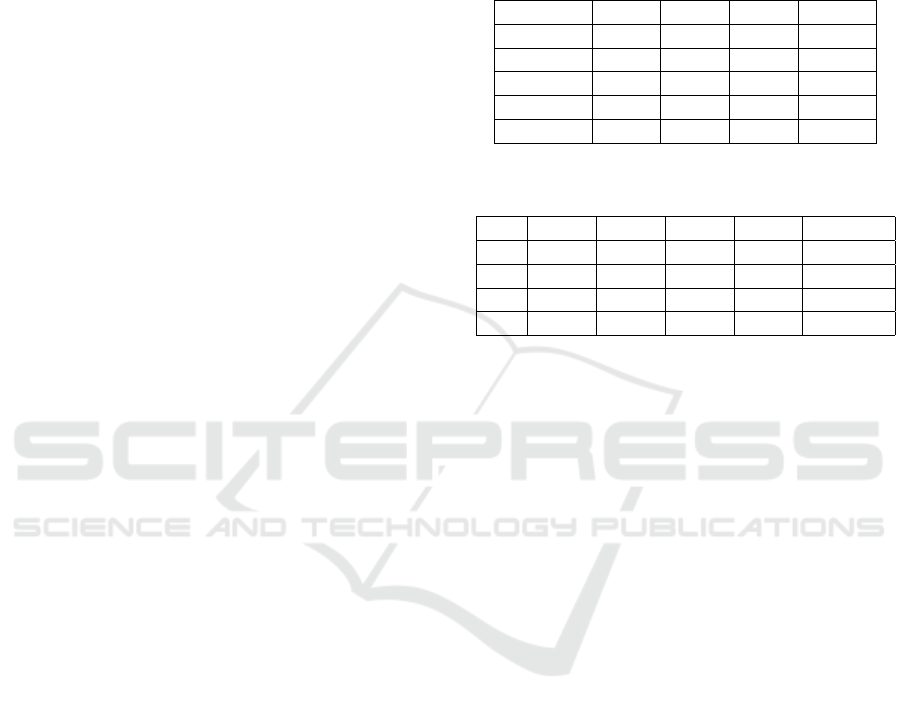
Table 5: An hypothetical database with 10 cloud providers, 4 PIs and 5 possible customer requests.
PI/Prov. Type P
1
P
2
P
3
P
4
P
5
P
6
P
7
P
8
P
9
P
10
RAM HB 4 2 8 4 2 8 16 4 2 8
Disc NB 10 20 30 25 40 30 20 20 15 20
Core HB 2 1 3 6 4 2 8 2 2 4
Cost LB 1,50 1,25 3,00 2,50 2,75 2,80 4,50 2,50 1,75 3,20
Customers Requests Set
PI/Request Request 1 Request 2 Request 3 Request 4 Request 5
PI Name Value Weight Value Weight Value Weight Value Weight Value Weight
RAM 4 1 2 1 8 1 16 1 16 0,5
Disc 20 1 10 1 30 1 20 1 40 0,25
Core 2 1 2 1 – – 3 1 3 0,25
known Optimal P8 P1 P6 P3 P7
First step is the calculation of DEA inputs
(“Resources” and “Costs”) and outputs (“Suitability”
and “Leftovers”), which done by Equations 4, 5, 6 and
7, where x
i j
is the PI value in database, X
j
the PI value
in request (customer desired one) and y
i
is the cost of
ith provider. To accomplish that, it is used data on the
database and requests in Table 5. Moreover, it is also
considered in the PIs conversion the following values:
α,β,δ = 1; γ = 2; Max(RAM) = 16; Max(Disc) = 40;
Max(Core) = 8; Min(Core) = 1; Max(cost) = 4,50;
n = 10; m = 3 (except for request 3, which is 2)
and each w
j
= 1 (except for request 5, where PI
“RAM” is two times more important that PI “Disc”
and “Core”, “Disc” is equally important as “Core”,
see Subsection 4.2 for more details).
Thus, Table 6 presents the final values for
inputs/outputs variables of DEA, as such the final
efficiency calculated by ISYDS using BCC model
with outputs orientation (according to Subsection 4.3)
for the requests 1, 2, 3, 4 and 5. In addition,
Table 6 have also the final ranking for each set of
efficient providers for each request, according the
described in Subsection 4.4. Note that the “Costs”
values remain constant for all requests, “Resources”
values are equals for requests 1 and 2, “Leftovers”
values for request 5 is all filled with zeros and will be
ignored by DEA as a valid output, and finally, that all
inputs/outputs are in the closed range between 0 and
1, including provider’s efficiency, as expected.
Analyzing Table 6 it is possible to identify the
providers that form the efficiency frontier for each
request. For request 1, providers P
1
&P
2
have lower
“Costs”, P
5
&P
7
have higher “Leftovers” and P
6
&P
8
have higher “Suitability”. The efficient providers in
request 2 are P
1
&P
6
&P
8
&P
9
(higher “Suitability”),
P
2
(lower “Costs”) and P
7
(higher “Leftovers”). For
request 3, P
3
&P
6
(higher “Suitability”) and P
5
&P
7
(higher “Leftovers”). For request 4, P
2
(lower
“Costs”), P
3
&P
7
(higher “Suitability”) and P
5
(higher
“Leftovers”). Finally, for request 5, P
7
(higher
“Suitability”) and P
3
(because it has low “Resources”
and is average in “Suitability”) are the efficient ones.
The final ranking can be obtained by analyzing only
values of “Suitability” and “Costs”. Thus, according
to the ranking, the best providers to attend each
request are: P
8
(Request 1), P
1
(Request 2), P
6
(Request 3), P
3
(Request 4), P
7
(Request 5), exactly
as expected in Table 5. For this small scenario, with
only ten providers, DEA removed very few providers
from ranking (except request 5), but for larger cases
with 100 or more providers, this quantity will be more
significant and DEA importance will be much more
evident.
6 FINAL CONSIDERATIONS
This work specified a mathematical model for
selecting and ranking cloud computing providers,
assisting customer decision making, using a
multi-criteria method called Data Envelopment
Analysis (DEA). The model is divided in three main
modules that are the DEA Input Converter, DEA
Method and Ranking Routine. This proposed model
is PI based, including PI types, values, desirable
values, tolerance and weights. It uses a provider
database and a customer request for calculating DEA
providers’ inputs and outputs, and then efficiency.
Finally, the proposed model performs the final
ranking on the selected cloud providers, using the
same DEA inputs and outputs.
The proposed model can use all kinds of
quantitative PIs plus the cost as a PI to operates.
DEA use inputs and outputs criteria to calculate
efficiency. The input criteria identified in this paper
are “Resources” and “Costs”, to be minimized. The
outputs criteria are “Suitability” and “Leftovers”.
All these criteria are normalized between 0 and 1.
The most important criteria is “Suitability”, followed
by “Costs”, “Leftovers” and “Resources”. An
ICEIS 2018 - 20th International Conference on Enterprise Information Systems
552

Table 6: Calculation of DEA inputs/outputs, efficiency and final rank for each cloud provider for each request.
Request 1
DMU Resources Costs Suitability Leftovers Efficiency Rank Optimal
P
1
0,5 0,333 0,444 0 1 3 –
P
2
0,506 0,278 0,111 0 1 5 –
P
3
0,298 0,667 0,444 0,417 0,935 – –
P
4
0,565 0,556 0,444 0,125 0,494 – –
P
5
0,387 0,611 0,111 0,5 1 6 –
P
6
0,25 0,622 1 0,417 1 2 –
P
7
0,452 1 0,444 0,5 1 4 –
P
8
0,417 0,556 1 0 1 1 P8
P
9
0,5 0,389 0,111 0 0,190 – –
P
10
0,429 0,711 0,444 0,167 0,444 – –
Request 2
P
1
0,5 0,333 1 0,071 1 1 P1
P
2
0,506 0,278 0,444 0,167 1 5 –
P
3
0,298 0,667 0,444 0,548 0,975 – –
P
4
0,565 0,556 0,444 0,322 0,678 – –
P
5
0,387 0,611 0,444 0,5 0,934 – –
P
6
0,25 0,622 1 0,548 1 4 –
P
7
0,452 1 0,444 0,667 1 6 –
P
8
0,417 0,556 1 0,238 1 3 –
P
9
0,5 0,389 1 0,083 1 2 –
P
10
0,429 0,711 0,444 0,381 0,662 – –
Request 3
P
1
0,75 0,333 0 0 0 – –
P
2
0,688 0,278 0 0 0 – –
P
3
0,375 0,667 1 0 1 2 –
P
4
0,562 0,556 0 0 0 – –
P
5
0,438 0,611 0,25 0,5 1 3 –
P
6
0,375 0,622 1 0 1 1 P6
P
7
0,25 1 0,25 0,5 1 4 –
P
8
0,625 0,556 0 0 0 – –
P
9
0,75 0,389 0 0 0 – –
P
10
0,5 0,711 0,25 0 0,25 – –
Request 4
P
1
0,548 0,333 0 0 0 – –
P
2
0,554 0,278 0,111 0 1 3 –
P
3
0,25 0,667 0,444 0,25 1 1 P3
P
4
0,518 0,556 0,111 0,125 0,447 – –
P
5
0,339 0,611 0,111 0,5 1 4 –
P
6
0,298 0,622 0,111 0,25 0,829 – –
P
7
0,405 1 0,444 0 1 2 –
P
8
0,464 0,556 0,111 0 0,318 – –
P
9
0,548 0,389 0 0 0 – –
P
10
0,381 0,711 0,111 0 0,25 – –
Request 5
P
1
0,598 0,333 0 0 0 – –
P
2
0,634 0,278 0 0 0 – –
P
3
0,312 0,667 0,0625 0 1 2 –
P
4
0,576 0,556 0 0 0 – –
P
5
0,473 0,611 0,0625 0 0,562 – –
P
6
0,348 0,622 0 0 0 – –
P
7
0,304 1 0,25 0 1 1 P7
P
8
0,536 0,556 0 0 0 – –
P
9
0,629 0,389 0 0 0 – –
P
10
0,411 0,711 0 0 0 – –
An Efficiency Frontier based Model for Cloud Computing Provider Selection and Ranking
553

example case was solved using the proposed model,
demonstrating its use and results of its adoption.
Future work includes testing the proposed model
for larger problems (more than 100 provider and more
PIs) and with realistic settings (real providers and real
data), as well as the creation of a cloud computing
selection framework with multiple selection methods
that incorporates this DEA method. Also, it is
expected to improve the model in order to handle
qualitative PIs.
REFERENCES
Achar, R. and Thilagam, P. (2014). A broker based appro-
ach for cloud provider selection. In 2014 International
Conference on Advances in Computing, Communica-
tions and Informatics (ICACCI), pages 1252–1257.
Baranwal, G. and Vidyarthi, D. P. (2014). A framework for
selection of best cloud service provider using ranked
voting method. In Advance Computing Conference
(IACC), 2014 IEEE International, pages 831–837.
Charnes, A., Cooper, W., and Rhodes, E. (1978). Measu-
ring the efficiency of decision making units. European
Journal Of Operational Research, 2(6):429–444.
Cook, W. and Kress, M. (1990). A data envelopment mo-
del for aggregating preference rankings. Management
Science, 36(11):1302–1310.
CSMIC (2014). Service measurement index framework.
Technical report, Carnegie Mellon University, Silicon
Valley, Moffett Field, California. Accessed in Novem-
ber 2016.
Garg, S. K., Versteeg, S., and Buyya, R. (2013). A frame-
work for ranking of cloud computing services. Future
Generation Computer Systems, 29:1012–1023.
Hogan, M. D., Liu, F., Sokol, A. W., and Jin, T. (2013). Nist
Cloud Computing Standards Roadmap. NIST Special
Publication 500 Series. accessed in September 2015.
Hwang, C.-L. and Yoon, K. (1981). Methods for multiple
attribute decision making. In Multiple attribute deci-
sion making, pages 58–191. Springer.
Ishizaka, A. and Nemery, P. (2013). Multi-Criteria Decision
Analysis: Methods and Software. John Wiley & Sons,
Ltd, United Kingdom.
Jain, R. (1991). The Art of Computer Systems Performance
Analysis: Techniques for Experimental Design, Mea-
surement, Simulation, and Modeling. John Wiley &
Sons, Littleton, Massachusetts.
Jaiswal, A. and Mishra, R. (2017). Cloud service selection
using topsis and fuzzy topsis with ahp and anp. In
Proceedings of the 2017 International Conference on
Machine Learning and Soft Computing, pages 136–
142. ACM.
Li, A., Yang, X., Kandula, S., and Zhang, M. (2010). Clou-
dcmp: comparing public cloud providers. In Procee-
dings of the 10th ACM SIGCOMM conference on In-
ternet measurement, pages 1–14. ACM.
Meza, L. A., Neto, L. B., Soares-Mello, J., and Gomes, E.
(2005). Isyds integrated system for decision support
(siad sistema integrado de apoio a decisao): a soft-
ware package for data envelopment analysis model.
Pesquisa Operacional, 25(3):493–503.
Moraes, L., Fiorese, A., and Matos, F. (2017). A multi-
criteria scoring method based on performance indica-
tors for cloud computing provider selection. In 19th
International Conference on Enterprise Information
Systems (ICEIS 2017), volume 2, pages 588–599.
Ramanathan, R. (2003). An Introduction to Data Envelop-
ment Analysis: A Tool for Performance Measurement.
Sage Publications, Ltd, London.
Saaty, T. L. (1990). How to make a decision: The analytic
hierarchy process. European Journal of Operational
Research, 48:9–26.
Saaty, T. L. (2004). Decision making – the analytic hier-
archy and network processes (ahp/anp). Journal of
Systems Science and Systems Engineering, 13:1–35.
Shirur, S. and Swamy, A. (2015). A cloud service measure
index framework to evaluate efficient candidate with
ranked technology. International Journal of Science
and Research, 4.
Sodhi, B. and T V, P. (2012). A simplified description of
fuzzy topsis. arXiv preprint arXiv:1205.5098.
Sundareswaran, S., Squicciarin, A., and Lin, D. (2012).
A brokerage-based approach for cloud service se-
lection. In 2012 IEEE Fifth International Conference
on Cloud Computing, pages 558–565.
Wagle, S., Guzek, M., Bouvry, P., and Bisdorff, R. (2015).
An evaluation model for selecting cloud services from
commercially available cloud providers. In 7th Inter-
national Conference on Cloud Computing Technology
and Science, pages 107–114.
Whaiduzzaman, M., Gani, A., Anuar, N. B., Shiraz, M., Ha-
que, M. N., and Haque, I. T. (2014). Cloud service
selection using multicriteria decision analysis. The
Scientific World Journal, 2014.
Zhang, Q., Cheng, L., and Boutaba, R. (2010). Cloud com-
puting: state-of-the-art and research challenges. Jour-
nal of Internet Services and Applications, 1:7–18.
Zhou, M., Zhang, R., Zeng, D., and Qian, W. (2010). Ser-
vices in the cloud computing era: A survey. Universal
Communication Symposium (IUCS), 2010 4th Inter-
national, pages 40–46.
ICEIS 2018 - 20th International Conference on Enterprise Information Systems
554