
Optimal Time-sampling Problem in a Statistical Control
with a Quadratic Cost Functional
Analytical and Numerical Approaches
Valery Y. Glizer and Vladimir Turetsky
Department of Applied Mathematics, ORT Braude College of Engineering, P. O .B. 78, Karmiel 2161002, Israel
Keywords:
Statistical Control, Statistical Information, Quadratic Cost Functional, Optimal Time-sampling, Pontryagin’s
Maximum Principle, Quadratic Optimization.
Abstract:
We consider the problem of constructing an optimal time-sampling for a Statistical Process Control (or, briefly,
Statistical Control (SC)). The aim of this time-sampling is to minimize the expected loss, caused by a delay
in the detection of an undesirable process change. We study the case where this loss is a quadratic functional
of the sampling time-interval. This problem is modeled by a nonstandard calculus of variations problem.
We propose two approaches to the solution of this calculus of variations problem. The first approach is
based on its equivalent transformation to an optimal control problem. The latter is solved by application
of the Pontryagin’s Maximum Principle, yielding an analytical expression for the optimal time-sampling in
the SC. The second approach uses a discretization of the calculus of variations problem, resulting in a finite
dimensional quadratic optimization problem. Solution of the latter provides a suboptimal time-sampling in
the SC. The time-samplings, obtained by these two approaches, are compared to each other in numerical
examples.
1 INTRODUCTION
The Statistical Control is a quality control method
(see, e.g., (Qiu, 2013) and references therein). It con-
sists in a monitoring of a process state using a statisti-
cal information on samples of its characteristic index
in some time-intervals. The SC is applied in indu-
stry, medicine, veterinary, environment control, etc.
Its objective is to minimize losses which can be cau-
sed by delay in the detection of undesirable process
changes, subject to reasonable inspection expenses.
For many years, the traditional SC practice was to
take samples of the process characteristic index with
a fixed time-sampling. The idea of using a variable
time-sampling (VTS) in the SC was suggested for the
first time in the work (Reynolds et al., 1988). Then,
this idea was developed in a number of works (see,
e.g., (Amin and Hemasinha, 1993); (Amin and Miller,
1993); (Bashkansky and Glizer, 2012); (Chew et al.,
2015); (Costa, 1994); (Costa, 1997); (Costa, 1998);
(Costa, 1999b); (Costa, 1999a); (Costa and Magal-
haes, 2007); (Glizer et al., 2015); (Hatjimihail, 2009);
(Sultana et al., 2014); (Li and Qiu, 2014); (Prabhu
et al., 1994); (Reynolds, 1995)).
In (Reynolds et al., 1988), the delay in the de-
tection of a process change was considered as a cri-
terion for optimality of the variable sampling time-
interval in the SC. Another possible criterion, propo-
sed in (Taguchi et al., 2007). is the expected loss due
to such a delay. The latter criterion is more general
and, therefore, more suitable for various applications.
In many processes, the relation between the ex-
pected loss and the delay in the detection of a process
change is non-linear. Among such processes, we can
mention: (i) fires propagation (Babrauskas, 2008), (ii)
oil spills spreading (Sebasti˜ao and Soares, 1995), (iii)
cholesterol plaque growth (Bulelzai and Dubbeldam,
2012), (iv) epidemics propagation (Carpenter et al.,
2011), (v) fatigue crack growth in ship hull structures
(Kim and Frangopol, 2011).
Genichi Taguchi (see e.g. (Taguchi et al., 2007))
proposed a quadratic dependence of the expected loss
on some critical performance parameter of a process.
In modern industry, medicine, veterinary, natural en-
vironment protection, etc, the statistical control of a
process becomes its indispensable part. Therefore,
the delay in the detection of a process change can be
considered as a critical performance parameter of the
process. This observation yields a quadratic depen-
dence of the expected loss on the detection delay.
Glizer, V. and Turetsky, V.
Optimal Time-sampling Problem in a Statistical Control with a Quadratic Cost Functional - Analytical and Numerical Approaches.
DOI: 10.5220/0006829000210032
In Proceedings of the 15th International Conference on Informatics in Control, Automation and Robotics (ICINCO 2018) - Volume 1, pages 21-32
ISBN: 978-989-758-321-6
Copyright © 2018 by SCITEPRESS – Science and Technology Publications, Lda. All rights reserved
21

We model the problem of the SC time-sampling
optimization by some calculus of variations problem.
This problem consists of a cost functional (the ex-
pected loss) and two types of constraints (geome-
tric and integral inequality constraints). The geo-
metric constraint gives the lower and upper bounds
of each sampling time-interval. The integral inequa-
lity constraint means that the average of the sampling
time-interval is not prescribed but it belongs to a gi-
ven interval. This model for the SC time-sampling
optimization is more general than those studied in
((Bashkansky and Glizer, 2012); (Glizer et al., 2015)).
Moreover, both types of the constraints are not studied
in the classical calculus of variations theory. Thus, the
considered extremal problem is nonstandard. We pro-
pose two methods of its solution, which are not based
on a preliminary approximate decomposition of this
problem. The first method converts equivalently the
original extremal problem into an optimal control pro-
blem. This optimal control problem is solved using
the Pontryagin’s Maximum Principle (PMP), which
yields an exact analytical solution to the original cal-
culus of variations problem. This solution constitutes
the optimal time-sampling of the SC. In the second
method, the original calculus of variations problem is
replaced approximately with a finite-dimensional op-
timization problem. The latter is solved using cor-
responding mathematical programming tools, which
yields an approximate solution of the original extre-
mal problem. This solution constitutes the su boptimal
time-sampling of the SC.
It is important to note, that the SC time-sampling,
designed in this paper, depends on the current state of
the process. It is not designed in advance for an en-
tire period of the process control. Applying the termi-
nology of control engineering, this SC time-sampling
can be called a state-feedback time-sampling.
Also, it should be noted that in most VTS sche-
mes, described in the literature, the sampling time-
interval of only two different lengths is considered. In
the present paper, as well as in (Li and Qiu, 2014) and
(Glizer et al., 2015), more than two different lengths
of the sampling time-interval are proposed for the SC.
In (Li and Qiu, 2014), the multiple lengths sampling
time-interval is related to the p-value of the charting
statistic, while in (Glizer et al., 2015) and the present
paper, such sampling time-intervals are derived from
solutions (exact and approximate) of the optimization
problems.
2 PROBLEM STATEMENT
We analyze the SC case where the monitoring of a
characteristic index x of the process state is carried out
based on the information about its sample mean. Na-
mely, at some prescribed/precalculated time instance
t a batch of n observations x
j
, (j =
1,n) of the value x
is obtained, and the sample mean ¯x of these observati-
ons is derived. We assume that the sample size n is in-
dependent of t. Let µ and σ be the mean value and the
standard deviation of the random value x. Then, the
mean value and the standard deviation of the random
value ¯x are µ and σ/
√
n. In this paper, we deal with
the case where the random value ¯x is normally distri-
buted, i.e., ¯x ∼ N(µ, σ/
√
n). This occurs when either
the random value x is normally distributed, or the
sample size n is considerably large (n ≥ 30). In the
latter case, by virtue of the Central Limit Theorem,
the normal distribution N(µ, σ/
√
n) provides a good
approximation of ¯x even if x does not strictly fit a nor-
mal distribution (see, e.g., (Qiu, 2013) and references
therein). Thus, the normalized sample mean, called
the standard score, is z =
¯x−µ
/
σ/
√
n
∼N(0,1).
The upper and lower limits of the standard Shewhart
control chart for z are z
min
= −3 and z
max
= 3, re-
spectively, (see (Qiu, 2013)). Therefore, the false
alarm probability α (type I error), i.e., the probability
of the event z /∈ [−3, 3], is α ≈ 0.0027.
Let the mean value of the index x is shifted by ∆,
i.e., a new mean value is µ
′
= µ+∆, while the standard
deviation σ remains unchanged. Then the distribu-
tion of z becomes z ∼ N(δ,1), where the normalized
shift δ = ∆/
σ/
√
n
is the so-called signal-to-noise
ratio. The probability of discovering the shift (recei-
ving the signal) by a single sample is the probability
of the event z /∈ [−3, 3] for z ∼ N(δ,1):
1 −β = 1 −
1
√
2π
Z
3
−3
exp
−(z −δ)
2
/2
dz
= 1 −[Φ(3 −δ)−Φ(−3 −δ)], (1)
where β = β(δ) is the probability of a type II error
(not discovering the shift).
Consider the SC with a variable sampling time-
interval u(z), depending on the standard score z =
¯x −µ
/
σ/
√
n
. Since the value of the sampling
time-interval should depend only on |z|, the function
u(z) is even
u(−z) = u(z)
. Therefore, in what fol-
lows, we consider the function u(z) in the interval
[0,3]. Also, for the sake of simplicity, we assume that
δ ≥ 0. The case δ ≤0 is treated similarly. Further, we
assume that the function u(z) is bounded as:
0 < u
min
≤ u(z) ≤ u
max
, z ∈ [0,3]. (2)
The inequality (2) is a geometric constraint, imposed
ICINCO 2018 - 15th International Conference on Informatics in Control, Automation and Robotics
22

on the function u(z). Now, let us consider the follo-
wing integral constraint, imposed on u(z):
aT
min
≤
Z
3
0
exp(−z
2
/2)u(z)dz ≤ aT
max
, (3)
where 0 < T
min
< T
max
, and
a
△
=
Z
3
0
exp(−z
2
/2)dz > 0. (4)
Remark 1. The inequality (3) means that the ex-
pected sampling time-interval in the case of u nshif-
ted z (δ = 0) belongs to a prescribed nominal interval
[T
min
,T
max
]. We assume that
T
min
> u
min
, T
max
< u
max
. (5)
If the shift of the mean in the process characteris-
tic index remains constant, the time t
d
, required for
discovering this shift (so-called time to signal), is the
sum of a random amount K
d
of random independent
and identically distributed sampling time-intervals u
i
,
conditionally independent of K
d
: t
d
=
K
d
∑
i=1
u
i
. The va-
lue K
d
is distributed geometrically with the success
probability 1 −β, given by (1). Its mathematical ex-
pectation and variance are (Ross, 2009): E(K
d
) =
1/(1 −β), Var(K
d
) = β/(1 −β)
2
.
The cost functional, to be minimized by a proper
choice of the sampling time-interval u(z), is the mat-
hematical expectation E(L) of the loss L, caused by
the delay in the detection of the shift. Here, we con-
sider the loss L as a quadratic function of the delay
t
d
, i.e., L = kt
2
d
, where k = k(δ) ≥ 0 is an increasing
function of δ ≥ 0 and k(0) = 0. Thus, the expected
loss is
E(L) = k(δ)E(t
2
d
). (6)
By routine calculations, we have
E(t
2
d
) = A(δ)
Z
3
0
ψ(z,δ)u
2
(z)dz
+B(δ)
Z
3
0
ψ(z,δ)u(z)dz
2
, (7)
where
A(δ)
△
=
exp(−δ
2
/2)
(1 −β)β
√
2π
> 0, B(δ)
△
=
2 exp(−δ
2
/2)
(1 −β)
√
2π
> 0,
(8)
ψ(z,δ)
△
= 2exp
−z
2
/2
cosh(δz) > 0, z ∈[0,3]. (9)
Since k(δ) > 0 for all δ > 0, then due to (7) – (8),
the minimization of the cost functional (6) for any gi-
ven δ > 0 is equivalent to the minimization of the fol-
lowing cost functional:
J
u(z)
△
=
Z
3
0
ψ(z,δ)u
2
(z)dz
+B(δ)
Z
3
0
ψ(z,δ)u(z)dz
2
. (10)
Remark 2. Two cases can be distinguished with re-
spect to the information on the value of δ: (i) the value
of δ is known; (ii) the value of δ is unknown. In the
first case, one should minimize with respect to u(z) the
cost functio nal (10), calculated for the known δ. In
the second case, one should minimize with respect to
u(z) the cost functional (6) – (7) robustly in δ ≥0, i.e.,
one should minimize with respect to u(z) the new cost
functional J
new
u(z)
= max
δ≥0
k(δ)E(t
2
d
). In this pa-
per, we restrict our analysis with the first case.
Thus, we can formulate the following extremal
problem.
Extremal Problem (EP): for a known δ ≥ 0, to find
the function u(z), z ∈ [0,3], which minimizes the cost
functional (10) subject to the constraints (2), (3) and
the inequality (5).
In subsequent sections, we solve the EP in a closed
analytical form and numerically, thus designing the
optimal and suboptimal SC time-sampling.
3 ANALYTICAL SOLUTION OF
THE EP
The EP is a nonstandard calculus of variations pro-
blem with two types of constraints, the geometric con-
straint (2) and the integral inequality constraint (3),
imposed on the minimizing function. The classical
calculus of variations theory does not study extremal
problems with such types of constraints (see, e.g.,
(Gelfand and Fomin, 1963)). We propose another ap-
proach to the solution of this problem, which consists
in an equivalent transformation of the EP into an opti-
mal control problem. The latter is analyzed by appli-
cation of the control optimality necessary condition –
the Pontryagin’s Maximum Principle (PMP) (Pontry-
agin et al., 1962).
3.1 Transformation of the EP
Let us introduce the auxiliary vector-valued function
w(z) =
w
1
(z),w
2
(z),w
3
(z)
T
, z ∈ [0,3], where
w
1
(z) =
Z
z
0
ψ(ζ,δ)u
2
(ζ)dζ, (11)
w
2
(z) =
Z
z
0
ψ(ζ,δ)u(ζ)dζ, (12)
w
3
(z) =
Z
z
0
exp
−ζ
2
/2
u(ζ)dζ. (13)
The functions w
i
(z), (i = 1, 2, 3), satisfy the differen-
tial equations
dw
1
/dz = ψ(z,δ)u
2
(z), (14)
Optimal Time-sampling Problem in a Statistical Control with a Quadratic Cost Functional - Analytical and Numerical Approaches
23

dw
2
/dz = ψ(z,δ)u(z), (15)
dw
3
/dz = exp
−z
2
/2
u(z), (16)
and the initial conditions
w
1
(0) = 0, w
2
(0) = 0, w
3
(0) = 0. (17)
Based on (13), the integral inequality (3) of the EP
becomes
aT
min
≤ w
3
(3) ≤ aT
max
. (18)
This inequality can be rewritten equivalently as the set
of two inequalities
g
1
w(3)
△
= −w
3
(3) + aT
min
≤ 0, (19)
g
2
w(3)
△
= w
3
(3) −aT
max
≤ 0. (20)
Using (11) – (12), the cost functional (10) beco-
mes
J
u(z)
= w
1
(3) + B(δ)
w
2
(3)
2
. (21)
Thus, we have transformed the EP into the equi-
valent optimal control problem: to find the control
function u(z), transferring the system (14) – (16) from
the initial position (17) to the set of terminal positions
(19) – (20) and minimizing the cost functional (21),
subject to the geometric constraint (2) and the inequa-
lity (5). This optimal control problem is non-linear
with respect to u(z), and in what follows, it is cal-
led the Non-linear Optimal Control Problem (NOCP).
Due to (Ioffe and Tihomirov, 1979) (see Section 9.2,
Theorem 3), the NOCP has a solution (optimal cont-
rol).
3.2 Solution of the NOCP by
Application of the PMP
The Variational Hamiltonian of the NOCP is
H = H(w,u,λ,z)
= λ
1
ψ(δ,z)u
2
+ λ
2
ψ(δ,z)u + λ
3
exp
−z
2
/2
u, (22)
where λ = λ(z) =
λ
1
(z),λ
2
(z),λ
3
(z)
T
, and λ
i
=
λ
i
(z), (i = 1, 2, 3) are the costate variables. These co-
state variables satisfy the differential equations
dλ
1
/dz = −∂H/∂w
1
= 0, z ∈ [0,3], (23)
dλ
2
/dz = −∂H/∂w
2
= 0, z ∈ [0,3], (24)
dλ
3
/dz = −∂H/∂w
3
= 0, z ∈ [0,3], (25)
and the terminal conditions
λ
1
(3) = −C
0
∂J/∂w
1
(3)
= −C
0
, (26)
λ
2
(3) = −C
0
∂J/∂w
2
(3)
= −2C
0
B(δ)γ, γ
△
= w
2
(3),
(27)
λ
3
(3) = −C
0
∂J/∂w
3
(3)
−C
1
∂g
1
w(3)
/∂w
3
(3)
−C
2
∂g
1
w(3)
/∂w
3
(3)
= C
1
−C
2
. (28)
In these terminal conditions,
C
0
≥ 0, C
1
≥ 0, C
2
≥ 0 (29)
are some constants, such that
C
0
+C
1
+C
2
> 0, (30)
and
C
1
g
1
w(3)
= 0, C
2
g
2
w(3)
= 0. (31)
Denote I
u
△
=
u : u
min
≤ u ≤ u
max
. Due to the
PMP, an optimal control u
∗
(z) of the NOCP necessa-
rily satisfies the following condition for all z ∈ [0,3]:
max
u(z)∈I
u
H
w(z),u(z),λ(z),z
=
H
w(z),u
∗
(z),λ(z),z
. (32)
Thus, any control u(z), satisfying the equations (32),
(14) – (17) and (23) – (28), the conditions (19) –
(20) and (29) – (31), is an optimal control candi-
date in the NOCP. To obtain such a control, first, we
solve the equations (23) – (28). These equations yield
the following solution for z ∈ [0,3]: λ
1
(z) = −C
0
,
λ
2
(z) = − 2C
0
Bγ, λ
3
(z) = C
1
−C
2
. By substitution of
this solution into (22) and using (9), the Variational
Hamiltonian of the NOCP becomes
H = −exp
−z
2
/2
G
u,z,γ,C
0
,C
1
,C
2
, (33)
where the function G
u,z,γ,C
0
,C
1
,C
2
has the form
G
u,z,γ,C
0
,C
1
,C
2
=
4C
0
B(δ)γcosh(δz)−C
1
+C
2
u +
2C
0
cosh(δz)u
2
. (34)
Let us show that C
0
> 0. For this purpose, we assume
the opposite which, due to (29), is C
0
= 0. In this case,
the use of (33) – (34) and (30) yields
H = exp(−z
2
/2)(C
1
−C
2
)u (35)
and C
1
+C
2
> 0. Note that C
1
6= C
2
. Indeed, if C
1
=
C
2
, then both constants are non-zero. In such a case,
by virtue of (31), g
1
w(3)
= 0 and g
2
w(3)
= 0.
The latter, along with (19) – (20) and the inequality
T
min
< T
max
(see (5)), yields a contradiction. Thus,
C
1
−C
2
6= 0. The unique control, satisfying (32) with
the Variational Hamiltonian of the form (35) is
u
∗
(z) =
u
min
, if C
1
−C
2
< 0,
u
max
, if C
1
−C
2
> 0.
(36)
ICINCO 2018 - 15th International Conference on Informatics in Control, Automation and Robotics
24

Now, substituting (36) into (16) instead of u(z)
and solving the resulting equation subject to the initial
condition from (17), we obtain
w
3
(3) =
au
min
if C
1
−C
2
< 0,
au
max
, if C
1
−C
2
> 0.
(37)
The latter, along with the inequality (5), means that
w
3
(3) does not belong to the set of terminal positi-
ons (19) – (20). Therefore, the control (36), obtained
from (32), (35) under the assumption C
0
= 0, is not
admissible. This means that the assumption C
0
= 0 is
wrong, i.e., C
0
> 0.
Due to the PMP, we can set C
0
= 1 and rewrite the
equations (33) – (34) as:
H = −exp
−z
2
/2
G
1
u,z,γ,C
1
,C
2
, (38)
G
1
u,z,γ,C
1
,C
2
=
4B(δ)γcosh(δz)
−C
1
+C
2
u + 2 cosh(δz)u
2
. (39)
Thus, applying (32) to (38) – (39), we obtain the
optimal control of the NOCP in the form
u
∗
(z) = u
∗
(z,γ,C
1
,C
2
) =
u
min
, ˜u(z,γ,C
1
,C
2
) ≤ u
min
,
˜u(z,γ,C
1
,C
2
), ˜u(z,γ,C
1
,C
2
) ∈ (u
min
,u
max
],
u
max
, ˜u(z,γ,C
1
,C
2
) > u
max
,
(40)
where
˜u(z,γ,C
1
,C
2
) =
C
1
−C
2
/
4 cosh(δz)
−Bγ (41)
is the unique solution of the following equation with
respect to u: ∂G
1
(u,z,γ,C
1
,C
2
)/∂u = 0.
In order to use the equation (40), we need to know
the constants γ, C
1
and C
2
. These constants should be
chosen in such a way that the resulting control (40)
will transfer the system (14) – (16) from the initial
position (17) to the intersection of the set of termi-
nal positions (19) – (20) and the plane w
2
(3) −γ = 0
in the 3D-space
w
1
(3),w
2
(3),w
3
(3)
. Substituting
(40) into the system (14) – (16) instead of u(z), sol-
ving the resulting system subject to the initial conditi-
ons (17), and using the above mentioned requirement
yield the following set of the inequality and the alge-
braic equation with respect to γ, C
1
and C
2
:
aT
min
≤ Φ
1
(γ,C
1
,C
2
) ≤ aT
max
, (42)
Φ
2
(γ,C
1
,C
2
) −γ = 0, (43)
where
Φ
1
(γ,C
1
,C
2
)
△
=
Z
3
0
exp(−z
2
/2)u
∗
(z,γ,C
1
,C
2
)dz,
(44)
Φ
2
(γ,C
1
,C
2
)
△
=
Z
3
0
ψ(z,δ)u
∗
(z,γ,C
1
,C
2
)dz. (45)
Note that Φ
1
(γ,C
1
,C
2
) and Φ
2
(γ,C
1
,C
2
) are the va-
lues w
3
(3) and w
2
(3), generated by the control (40).
Further, due to (19) – (20) and (31), the constants
γ, C
1
and C
2
should satisfy the algebraic equations
C
1
aT
min
−Φ
1
(γ,C
1
,C
2
)
= 0, (46)
C
2
Φ
1
(γ,C
1
,C
2
) −aT
max
= 0. (47)
Moreover, by (29),
C
1
≥ 0, C
2
≥ 0. (48)
Remark 3. Since the NOCP has the solution, the set
(42) – (48) has a solution. If this set has more th an
one solution, we choose the solution
γ = γ
∗
,C
1
=
C
∗
1
,C
2
= C
∗
2
, which provides the minimum value of
the NOCP cost functional (21) in c omparison with the
other solutions.
3.3 Analysis of the Set (42) – (48)
Let (γ,C
1
,C
2
) be a solution of this set. Since the
control (40) satisfies the inequality u
∗
(z,γ,C
1
,C
2
) ≥
u
min
> 0 for all z ∈ [0, 3], then due to (9), (43) and
(45), γ > 0. For the further analysis, we distinguish the
following cases with respect to C
1
and C
2
: (I) C
1
> 0,
C
2
> 0; (II) C
1
= C
2
= 0; (III) C
1
= 0, C
2
> 0; (IV)
C
1
> 0, C
2
= 0.
We start with the first case. Due to (46)-(47), this
case yields the contradictory equality aT
min
= aT
max
,
meaning that the first case is impossible.
Proceed to the second case. In this case,
the function ˜u(z,γ,C
1
,C
2
) (see (41)) becomes
˜u(z,γ,C
1
,C
2
) = ˜u(z,γ, 0, 0) = −B(δ)γ, z ∈[0,3]. Since
B(δ) and γ are positive, then ˜u(z,γ,C
1
,C
2
) < 0, z ∈
[0,3]. Therefore, due to the equation (40) and the
inequality u
min
> 0, we have u
∗
(z,γ,C
1
,C
2
) = u
min
,
z ∈ [0,3]. Now, substitution of this control into (44),
and using (42) and the positiveness of a yield the in-
equality T
min
≤ u
min
, which contradicts the inequality
in (5). Thus, the second case also is impossible.
Now, let us treat the third case. In this
case, we have ˜u(z,γ,C
1
,C
2
) = ˜u(z,γ,0,C
2
) =
−
C
2
/
4 cosh(δz)
+ B(δ)γ
< 0, z ∈ [0,3]. Thus, by
the same arguments as in the case (II), the third case
is impossible.
Finally, let us consider the case (IV). In this case,
by denoting C
△
= C
1
, the optimal control (40) becomes
u
∗
(z) = u
∗
(z,γ,C) =
u
min
, ¯u(z,γ,C) ≤ u
min
,
¯u(z,γ,C), u
min
< ¯u(z,γ,C) ≤ u
max
,
u
max
, ¯u(z,γ,C) > u
max
,
(49)
where
¯u(z,γ,C) = C/
4 cosh(δz)
−B(δ)γ (50)
Optimal Time-sampling Problem in a Statistical Control with a Quadratic Cost Functional - Analytical and Numerical Approaches
25

is the unique solution of the following equation with
respect to u: ∂G
2
(u,z,γ,C)/∂u = 0, G
2
u,z,γ,C
=
4B(δ)γcosh(δz) − C
u + 2 cosh(δz)u
2
. Moreover,
using the equation (46) and denoting T
△
= T
min
, the
set (42) – (43) becomes
Λ
1
(γ,C)
△
=
Z
3
0
exp(−z
2
/2)u
∗
(z,γ,C)dz −aT = 0,
(51)
Λ
2
(γ,C)
△
=
Z
3
0
ψ(z,δ)u
∗
(z,γ,C)dz −γ = 0. (52)
Thus, to construct the optimal control u
∗
(z,γ,C)
and to design the optimal SC sampling time-interval,
one should solve the system (51) – (52) with respect
to (γ,C) and substitute its solution into the equation
(49). Due to Remark 3, the system (51) – (52) has a
solution. Some properties of this solution, helpful for
its numerical obtaining, are presented in the next sub-
section. Examples of such an obtaining are presented
in Section 5.
Remark 4. It is important to note that in the optimal
control u
∗
(z,γ,C) of the NOCP both bounds u
min
and
u
max
of the geometric con straint (2) are used. At the
same time, only the lower bound T
min
of the terminal
state inequality (18), equ iv alent to the integral ine-
quality (3), is used in the optimal control of the NOCP.
Thus, the optimal SC time-sampling depends on both
bounds of the geometric constraint (2) and only on the
lower bound of the integral inequality constraint (3).
3.4 Properties of the Solution to the
System (51) – (52)
Let us introduce into the consideration the following
values:
C
min
(γ)
△
= 4
B(δ)γ+ u
min
,
C
max
(γ)
△
= 4 cosh(3δ)
B(δ)γ+ u
max
,
γ
min
△
= u
min
Z
3
0
ψ(z,δ)dz, γ
max
△
= u
max
Z
3
0
ψ(z,δ)dz,
Γ
min
△
= max {γ
min
, 2aT },
Γ
max
△
= min{γ
max
, 2aT cosh(3δ)}.
Also, in the plane (γ,C), we consider the non-empty
domain
Ω
△
=
n
γ ∈
Γ
min
,Γ
max
,C ∈
C
min
(γ),C
max
(γ)
o
.
Based on the above introduced values and domain,
we obtain the following assertions.
Assertion 1. Let δ > 0. Let (γ,C) be a solution of the
system (51) – (52). Then, (γ,C) ∈ Ω.
Remark 5. Due to Assertion 1, in the case δ > 0, we
can look for the solution of the system (51) – (52) not
in the entire plane (γ,C), but in the bounded domain
Ω, which decreases considerably the computatio nal
effort. In the particular case of δ = 0, we can solve
the system (51) – (52) analytically.
Assertion 2. Let δ = 0. Then, the system (51) –
(52) has the unique solution
γ = 2aT,C = 8B(0)aT +
4T
.
Assertion 3. For any given δ > 0 and γ ∈
Γ
min
,Γ
max
, the equation (51) has the unique solu-
tion C =
e
C(γ), and
e
C(γ) ∈
C
min
(γ),C
max
(γ)
. (53)
Moreover,
e
C(γ) is a monotonically increasing
function of γ ∈
Γ
min
,Γ
max
.
Assertion 4. For any given δ > 0 and γ ∈
Γ
min
,Γ
max
, the equation (52) has the unique solu-
tion C =
¯
C(γ), and
¯
C(γ) ∈
C
min
(γ),C
max
(γ)
. (54)
Moreover,
¯
C(γ) is a monotonically increasing
function of γ ∈
Γ
min
,Γ
max
.
Remark 6. Based on Assertions 3 and 4, the γ-
compon ent of th e solution to the system (51) – (52)
can be obtained by solving with respect to γ ∈
Γ
min
,Γ
max
either the equation Λ
2
γ,
e
C(γ)
= 0, or
the equation Λ
1
γ,
¯
C(γ)
= 0, or the equation
e
C(γ) =
¯
C(γ).
The proofs of Assertions 1 – 4 are presented in
Appendix.
4 APPROXIMATE NUMERICAL
SOLUTION OF EP
Let us divide the interval [0,3] into N equal subinter-
vals by the collocation points
z
i
= i∆z, i = 0,1,.. .,N, ∆z = 3/N. (55)
Then, based on (55) and using the left rectangles for-
mula (Davis and Rabinowitz, 2007), we approximate
the integrals in the cost functional (10) and in the in-
tegral constraint (3).
Thus, the cost functional is approximated as:
J
u(z)
≈
˜
J
N
(U)
△
= ∆z
N−1
∑
i=0
ψ(z
i
,δ)U
2
i
+B
∆z
N−1
∑
i=0
ψ(z
i
,δ)U
i
!
2
, (56)
ICINCO 2018 - 15th International Conference on Informatics in Control, Automation and Robotics
26
where the vector U ∈E
N
is
U =
U
0
,U
1
,. . .,U
N−1
T
=
u(z
0
),u(z
1
),. .. ,u(z
N−1
)
T
. (57)
The constraint (3) is approximated as:
∆zT
min
N−1
∑
i=0
exp(−z
2
i
/2) ≤ ∆z
N−1
∑
i=0
exp(−z
2
i
/2)U
i
≤ ∆zT
max
N−1
∑
i=0
exp(−z
2
i
/2). (58)
The approximation (58) of the constraint (3) is de-
rived using the following approximation of the value
a:
a ≈ a
N
∆z, a
N
△
=
N−1
∑
i=0
exp(−z
2
i
/2).
The geometric constraint (2), appearing in the EP,
is approximated as:
u
min
≤U
i
≤ u
max
, i = 0, 1, ...,N −1. (59)
Dividing the expression in the right-hand side of
(56) and the inequality (58) by ∆z, we obtain the fol-
lowing finite-dimensional cost functional and the con-
straint:
J
N
(U)
△
=
N−1
∑
i=0
ψ(z
i
,δ)U
2
i
+B∆z
N−1
∑
i=0
ψ(z
i
,δ)U
i
!
2
, (60)
a
N
T
min
≤
N−1
∑
i=0
exp(−z
2
i
/2)U
i
≤ a
N
T
max
. (61)
Now, based on (60) – (61), we can formulate the
following quadratic programming problem.
Quadratic Programming Problem (QPP):
for a known δ ≥ 0, to find the vector
U =
U
0
,U
1
,...,U
N−1
T
which minimizes the
cost functional (60) subject to the constraints (59),
(61) and the inequality (5).
The QPP can be solved using standard optimiza-
tion tools, for example, the MATLAB function “quad-
prog”. It is reasonable to expect that for a sufficiently
large N, the components U
i
, (i = 0, 1, ...,N −1) of the
QPP solution will be close to the corresponding va-
lues u
∗
(z
i
,γ
∗
,C
∗
) of the optimal control in the NOCP.
In such a case, the optimal value of the cost functional
(60) in the QPP multiplied by ∆z will be close to the
optimal value of the cost functional (21) in the NOCP.
5 NUMERICAL EVALUATION OF
THE OPTIMAL AND
SUBOPTIMAL SAMPLING
TIME-INTERVALS
For the numerical evaluation, the following two sets
of parameters are chosen:
(I) u
min
= 0.5, u
max
= 3.5;
(II) u
min
= 0.1, u
max
= 2.5.
5.1 Numerical Solution of the System
(51) – (52)
To obtain the sampling time-interval u
∗
(z,γ,C), the
system (51) – (52) was solved numerically. The
value of γ was calculated by application of the bi-
section algorithm to the equation
e
C(γ) =
¯
C(γ) for
γ ∈(Γ
min
,Γ
max
).
Using Assertions 3 and 4, the functions
e
C(γ) and
¯
C(γ) also were derived by the bisection method for
(γ,C) ∈ Ω.
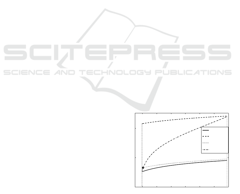
In Figs. 1 – 2, the functions
e
C(γ) and
¯
C(γ), along
with the functions C
min
(γ) and C
max
(γ), are depicted
in the logarithmic scale for the set (I) with δ = 2.5
(Fig. 1) and for the set (II) with δ = 2.9 (Fig. 2). The
value of T = T
min
= 1. It is seen that the functions
e
C(γ) and
¯
C(γ) are monotonically increasing, which
corresponds to the claims of Assertions 3 and 4. The
solution (γ,C) of the set (51) – (52), depicted by the
circle, belongs to the set Ω as it is stated in Assertion
1. Moreover, since the derivative of
¯
C(γ) with respect
to γ is larger than the derivative of
e
C(γ), this solution
is unique.
20 40 60 80 100 120 140
10
0
10
2
10
4
γ
C
Ω
Γ
min
Γ
max
C
min
(γ)
C
max
(γ)
e
C(γ)
¯
C(γ)
Figure 1:
e
C(γ),
¯
C(γ), C
min
(γ) and C
max
(γ): set (I).
The numerical solution (γ,C) of the set (51) –
(52), and the absolute values of the functions Λ
1
(γ,C)
Optimal Time-sampling Problem in a Statistical Control with a Quadratic Cost Functional - Analytical and Numerical Approaches
27
0 50 100 150 200
10
0
10
2
10
4
γ
C
Γ
min
Γ
max
Ω
C
min
(γ)
C
max
(γ)
e
C(γ)
¯
C(γ)
Figure 2:
e
C(γ),
¯
C(γ), C
min
(γ) and C
max
(γ): set (II).
and Λ
2
(γ,C) are presented in Table 1. It is seen that
the obtained numerical solution provides the deviati-
ons of Λ
1
(γ,C) and Λ
2
(γ,C) from zero smaller than
10
−4
.
Table 1: Numerical solution of (51) – (52).
Set δ γ C |Λ
1
(γ,C)| |Λ
2
(γ,C)|
(I) 2.5 21.1 20.6 2.9 ·10
−5
7.0 ·10
−5
(II) 2.9 12.6 13.4 7.1 ·10
−5
7.6 ·10
−5
5.2 Optimal Sampling Time-Interval
(EP Solution) vs. Approximate
Sampling Time-Interval (QPP
Solution)
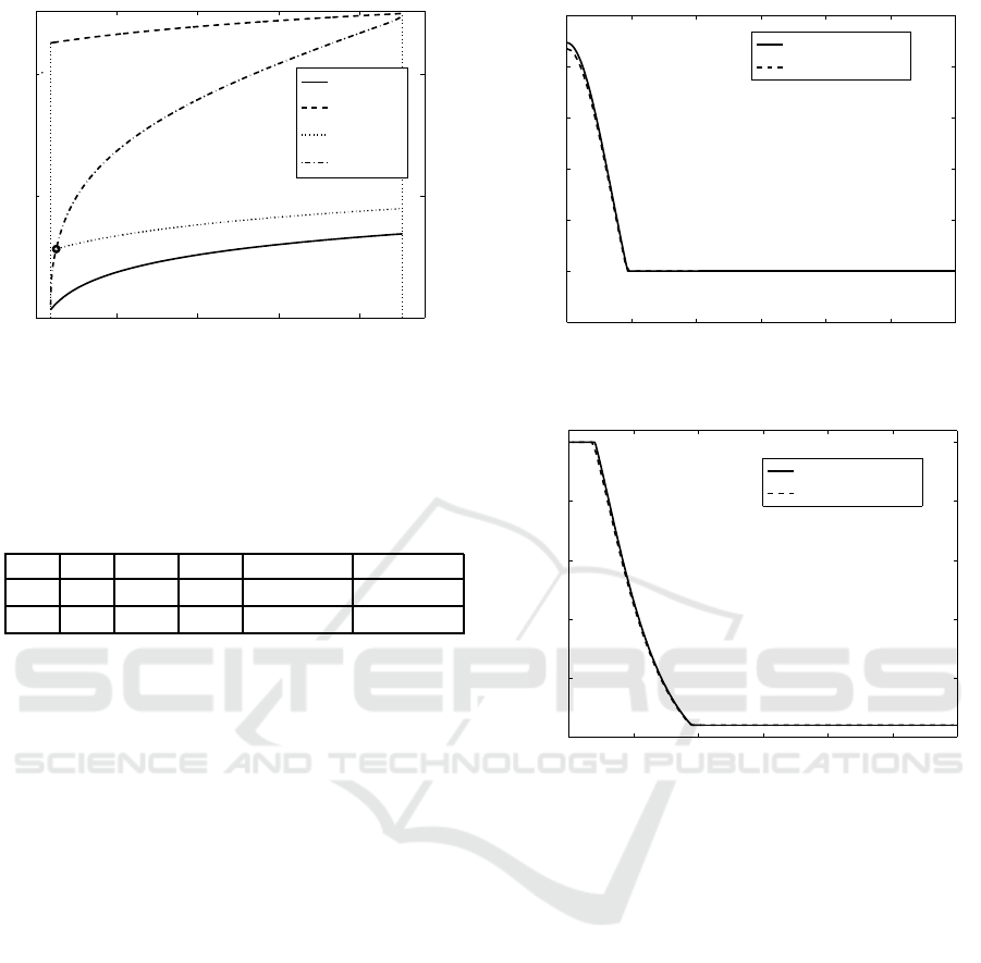
In Figs. 3 – 4, the optimal sampling time-interval
u
∗
(z,γ,C) (the EP solution), given by the analytical
expression (49), is compared to the approximate sam-
pling time-interval U
∗
(the QPP solution) for the set
(I) with δ = 2.5 (Fig. 3) and for the set (II) with
δ = 2.9 (Fig. 4). In both cases, T
min
= 1, T
max
= 2. It
is seen that the approximation, obtained for N = 100,
and the optimal sampling time-interval match well.
Note that in both cases, for the approximate so-
lution, the left-hand side inequality in the constraint
(61) is satisfied as the equality
N−1
∑
i=0
exp(−z
2
i
/2)U
i
= a
N
T
min
,
thus mimicking the corresponding property of the EP
analytical solution.
Based on the equation (49) and the above pre-
sented numerical calculations, the optimal sampling
time-interval for the set (I), depicted in Fig. 3, can be
rewritten as:
u
∗
(z,γ,C) =
¯u(z,γ,C), z ∈ [0,0.47),
u
min
, z ∈ [0.47,3].
0 0.5 1 1.5 2 2.5 3
0
0.5
1
1.5
2
2.5
3
z
u
∗
Optimal
Approximate
Figure 3: Optimal vs. approximate sampling time-interval:
set (I).
0 0.5 1 1.5 2 2.5 3
0
0.5
1
1.5
2
2.5
z
u
∗
Optimal
Approximate
Figure 4: Optimal vs. approximate sampling time-interval:
set (II).
The optimal sampling time-interval for the set (II), de-
picted in Fig. 4, can be rewritten in the form
u
∗
(z,γ,C) =
u
max
, z ∈ [0,0.21),
¯u(z,γ,C), z ∈ [0.21,0.95),
u
min
, z ∈ [0.95,3].
In Fig. 5, the optimal (minimum) value of the ex-
pected loss, given by (6)–(9), is depicted as a function
of δ for the set (I), T
min
= 1, and different coefficient
functions k = k(δ). It is seen that for each considered
k(δ), the optimal expected loss admits the maximum
for some value of δ, belonging to the interval (0,1).
6 CONCLUSIONS
In this paper, the problem of constructing an opti-
mal state-feedback sampling time-interval for the sta-
tistical control was considered. The expected loss,
quadratically dependent on the delay in the detection
of a process change, was chosen as the criterion of
ICINCO 2018 - 15th International Conference on Informatics in Control, Automation and Robotics
28
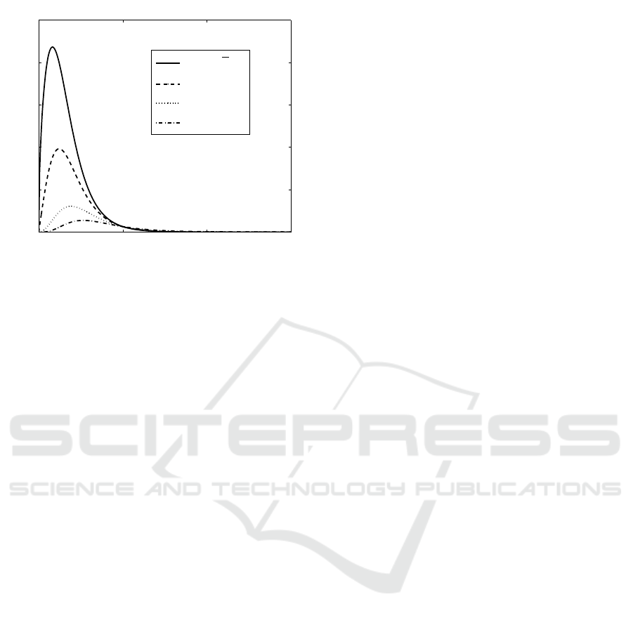
0 1 2 3
0
2
4
6
8
10
x 10
4
δ
Expected loss
k =
√
δ
k = δ
k = δ
2
k = δ
3
Figure 5: Optimal expected loss as a function of δ: set (I).
the optimization (minimization). This expected loss
also depends on the numerical parameter δ, characte-
rising a magnitude of the process change. The pro-
blem of the expected loss minimization was reduced
to the extremal problem in the form of a nonstan-
dard calculus of variations problem where the sam-
pling time-interval of the statistical control is a mini-
mizing function. This minimizing function depends
of the process state. Two methods of the solution of
this extremal problem were proposed. The first met-
hod transforms the original extremal problem to an
equivalent optimal control problem. Then, the latter
was solved using the Pontryagin’s Maximium Princi-
ple, which yields the explicit analytical expression for
the optimal sampling time-interval. This expression
contains two parameters. For obtaining these para-
meters, the set of two algebraic equations was derived
and analyzed. Based on this analysis, the method of
solution of this set was proposed. The second method
of the solution of the original extremal problem uses
its discretization. This leads to a finite-dimensional
extremal problem (the quadratic programming pro-
blem), approximating the original one. This qua-
dratic programming problem was solved using the
MATLAB function quadprog, providing the subopti-
mal sampling time-interval for the statistical control.
The optimal and suboptimal sampling time-intervals
were evaluated by numerical examples. This evalua-
tion has shown a good match of the optimal analytical
sampling time-interval and the suboptimal numerical
sampling time-interval. The optimal (minimum) va-
lue of the expected loss was constructed numerically
as a function of the parameter δ. It was shown that
this function has a single maximum.
It should be noted that the results, obtained in
this paper, are rather theoretical, and these results are
strongly based on two assumptions: (a) the sample
mean ¯x of the characteristic index x in the statistical
control is normally distributed; (b) the value of the
parameter δ, characterising a magnitude of the pro-
cess change, is known. Therefore, one can ask the
following: ”What will happen if at least one of these
assumptions is violated?” To answer this question, the
following issues will be studied in a future:
(I) an evaluation (by extensive computer simulations)
of the sampling time-interval, obtained in this paper,
in the cases where either a distribution of the sample
mean ¯x differs from the normal one, or the value of δ
is unknown;
(II) a design of optimal sampling time-interval in the
case where a distribution of the sample mean ¯x is not
normal;
(III) a design of optimal sampling time-interval, ro-
bust with respect to δ, in the case where the value of
this parameter is unknown.
Results of these studies will be presented in fort-
hcoming papers.
REFERENCES
Amin, R. W. and Hemasinha, R. (1993). The switching
behavior of
¯
X charts with variable sampling intervals.
Communication in Statistics - Theory and Methods,
22(7):2081–2102.
Amin, R. W. and Miller, R. W. (1993). A robustness study
of charts with variable sampling intervals. Journal of
Quality Technology, 25(1):36–44.
Babrauskas, V. (2008). Heat release rates. In SFPE Hand-
book of Fire Protection Engineering, pages 1–59. Na-
tional Fire Protection Association.
Bashkansky, E. and Glizer, V. Y. (2012). Novel appro-
ach to adaptive statistical process control optimiza-
tion with variable sampling interval and minimum ex-
pected loss. International Journal of Quality Engi-
neering and Technology, 3(2):91–107.
Bulelzai, M. A. K. and Dubbeldam, J. L. A. (2012). Long
time evolution of atherosclerotic plaques. Journal of
Theoretical Biology, 297:1–10.
Carpenter, T. E., OBrien, J. M., Hagerman, A., and McCarl,
B. (2011). Epidemic and economic impacts of delayed
detection of foot-and-mouth disease: a case study of a
simulated outbreak in california. Journal of Veterinary
Diagnostic Investi gation, 23(1):26–33.
Chew, X. Y., Khoo, M. B., Teh, S. Y., and Castagliola, P.
(2015). The variable sampling interval run sum
¯
X
control chart. Computers & Industrial Engineering,
90:25–38.
Costa, A. F. B. (1994). X charts with variable sample size.
Journal of Quality Technology, 26(3):155–163.
Costa, A. F. B. (1997).
¯
X charts with variable sample size
and sampling intervals. Journal of Quality Techno-
logy, 29(2):197–204.
Optimal Time-sampling Problem in a Statistical Control with a Quadratic Cost Functional - Analytical and Numerical Approaches
29

Costa, A. F. B. (1998). Joint
¯
X and r control charts with va-
riable parameters. IIE Transactions, 30(6):505–514.
Costa, A. F. B. (1999a).
¯
X charts with variable parameters.
Journal of Quality Technology, 31(4):408–416.
Costa, A. F. B. (1999b). Joint
¯
X and r charts with varia-
ble sample sizes and sampling intervals. Journal of
Quality Technology, 31(4):387–397.
Costa, A. F. B. and Magalhaes, M. S. D. (2007). An adap-
tive chart for monitoring the process mean and vari-
ance. Quality and Rel iability Engineering Internatio-
nal, 23(7):821–831.
Davis, P. J. and Rabinowitz, P. (2007). Methods of Nume-
rical Integration. Dover Publications Inc., Mineola,
NY.
Gelfand, I. M. and Fomin, S. V. (1963). Calculus of Varia-
tions. Prentice-Hall, Englewood Cliffs, NJ.
Glizer, V. Y., Turetsky, V., and Bashkansky, E. (2015).
Statistical process control optimization with varia-
ble sampling interval and nonlinear expected loss.
Journal of Industrial and Management Optimi zati on,
11(1):105–133.
Hatjimihail, A. T. (2009). Estimation of the optimal sta-
tistical quality control sampling time intervals using a
residual risk measure. PLoS ONE, 4(6):e5770.
Ioffe, A. D. and Tihomirov, V. M. (1979). Theory of Extre-
mal Problems. North-Holland Pub. Co., Amsterdam,
Netherlands.
Kim, S. and Frangopol, D. M. (2011). Optimum inspection
planning for minimizing fatigue damage detection de-
lay of ship hull structures. International Journal of
Fatigue, 33(3):448–459.
Li, Z. and Qiu, P. (2014). Statistical process control using
dynamic sampling. Technometrics, 56(3):325–335.
Pontryagin, L. S., Boltyanskii, V. G., Gamkrelidze, R. V.,
and Mishchenko, E. F. (1962). The Mathematical The-
ory of Optimal Processes. Interscience, New York,
NY.
Prabhu, S. S., Montgomery, D. C., and Runger, G. C.
(1994). A combined adaptive sample size and sam-
pling interval x control scheme. Journal of Quality
Technology, 26(3):164–176.
Qiu, P. (2013). Introduction to Statistical Process Control.
Chapman and Hall/CRC, Boca Raton, FL.
Reynolds, M. R. (1995). Evaluating properties of variable
sampling interval control charts. Sequential Analysis,
14(1):59–97.
Reynolds, M. R., Amin, R. W., Arnold, J. C., and Nachlas,
J. (1988).
¯
X charts with variable sampling intervals.
Technometrics, 30(2):181–192.
Ross, S. (2009). A First Course in Probability. Prentice
Hall, Upper Saddle River, NJ.
Sebasti˜ao, P. and Soares, C. G. (1995). Modeling the fate of
oil spills at sea. Spill Science and Technology Bulletin,
2(2-3):121–131.
Sultana, I., Ahmed, I., Chowdhury, A. H., and Paul, S. K.
(2014). Economic design of
¯
X control chart using
genetic algorithm and simulated annealing algorithm.
International Journal of Productivity and Quality Ma-
nagement, 14(3):352–372.
Taguchi, G., Chowdhury, S., and Wu, Y. (2007). Taguchi’s
Quality Engineering Handbook. John Wiley and Sons
Inc., Hoboken, NJ.
APPENDIX
The proofs of Assertions 1-4 are based on the follo-
wing auxiliary propositions.
Auxiliary Propositions
Proposition 1. For any given δ ≥ 0, there are no so-
lutions of the set (51) – (52) in the half-planes
C ≤C
min
(γ) (62)
and
C ≥C
max
(γ) (63)
of the plan e (γ,C).
Proof. First, let us prove the claim of the proposition
with respect to the half-plane (62), i.e., in the case
where the pair (γ,C) satisfies this inequality. In this
case, since cosh(δz) ≥ 1 for z ≥ 0, then ¯u(z,γ,C) ≤
u
min
for z ≥0. By virtue of (49), the latter means that
u
∗
(z,γ,C) = u
min
. Thus, due to (4), (5), (51), and the
notation T = T
min
,
Λ
1
(γ,C) = a
u
min
−T
< 0, (64)
meaning that the above mentioned pair (γ,C) does not
satisfy the equation (51). The claim of the assertion
with respect to the half-plane (63) is proven similarly.
Proposition 2. For any given δ ≥ 0, there are no so-
lutions of the set (51) – (52) in the half-planes
γ ≤γ
min
(65)
and
γ ≥γ
max
(66)
of the plan e (γ,C).
Proof. First of all, let us note the following. Since
0 < u
min
< u
max
and ψ(z,δ) > 0, z ∈ [0,3], then
0 < γ
min
< γ
max
. (67)
Consider the case where the pair (γ,C) satisfies the
strict inequality in (65). In this case, due to (9), (49),
(52) and (65), we have
Λ
2
(γ,C) >
Z
3
0
ψ(z,δ)
u
∗
(z,γ,C) −u
min
dz ≥ 0,
(68)
ICINCO 2018 - 15th International Conference on Informatics in Control, Automation and Robotics
30

meaning that (γ,C) does not satisfy the equation (52).
Now, let us consider the case γ = γ
min
. In this case,
using (49) and (52), we have
Λ
2
(γ
min
,C) =
Z
3
0
ψ(z,δ)
u
∗
(z,γ
min
,C) −u
min
dz ≥ 0. (69)
By virtue of (49), the inequality in (69) becomes
equality only if u
∗
(z,γ
min
,C) ≡ u
min
for all z ∈ [0,3],
yielding ¯u(z,γ
min
,C) ≤ u
min
for all z ∈ [0,3]. Using
(50), one directly obtains that the latter inequality for
z = 0 is equivalent to the inequality (62) with γ = γ
min
.
However, in this case by virtue of Proposition 1, the
equation (51) is not satisfied. Thus, the claim of the
assertion with respect to the half-plane (65) has been
proven. The claim of the proposition with respect to
the half-plane (66) is proven similarly.
Proposition 3. Let δ > 0. Let (γ,C) be a solution
of the set (51) – (52). Then, the component γ of this
solution satisfies the inequality
2aT < γ < 2aT cosh(3δ). (70)
Proof. Substitution of (9) into (52) yields after a sim-
ple rearrangement
γ = 2
Z
3
0
exp
−z
2
/2
cosh(δz)u
∗
(z,γ,C)dz. (71)
Applying the Mean Value Theorem to the integral in
the right-hand side of (71) and taking into account
the fact that cosh(δz) monotonically increases with
respect to z ∈ [0, 3] for δ > 0, we obtain
γ = 2 cosh(δ¯z)
Z
3
0
exp
−z
2
/2
u
∗
(z,γ,C)dz. (72)
where ¯z is some value from the interval (0, 3).
Due to (51), we can replace the integral in
(72) with aT , which leads to the equality γ =
2aT cosh(δ¯z). The latter, along with the inequality
1 < cosh(δ¯z) < cosh(3δ), directly implies the state-
ment of the proposition.
Proposition 4. For δ > 0, the following inequality
holds:
0 < Γ
min
< Γ
max
. (73)
Proof. Using the definition of γ
max
(see Subsection
3.4), the equation (4), the inequality (5), the notation
T = T
min
and the same arguments as in the proof of
Proposition 2, we obtain
γ
max
= 2au
max
cosh(δ˜z) > 2aT, (74)
where ˜z is some value from the interval (0, 3).
Similarly, using the definition of γ
min
(see Sub-
section 3.4), the equation (4) and the inequality (5),
we have
γ
min
= 2au
min
cosh(δ˜z) < 2aT cosh(3δ). (75)
Now, the inequalities (67), (74) and (75), along with
the inequality 2aT < 2aT cosh(3δ), yield immedia-
tely the statement of the proposition.
Proposition 5. For any γ ≥0, the following inequality
is valid:
0 < C
min
(γ) < C
max
(γ). (76)
Proof. The assertion directly follows from the defini-
tions of C
min
(γ) and C
max
(γ) (see Subsection 3.4).
Proof of Assertion 1
First of all let us note that, due to Propositions 4 and
5, the domain Ω indeed is non-empty. Now, the state-
ment of the assertion directly follows from Propositi-
ons 1-3 and the definitions of Γ
min
, Γ
max
and Ω.
Proof of Assertion 2
For δ = 0, the function ¯u
z,γ,C
, given by (50), beco-
mes a constant, i.e.,
¯u(z,γ,C) ≡
C
4
−B(0)γ, z ∈ [0, 3]. (77)
Moreover, due to Proposition 1, in order to be a solu-
tion of the set (51) – (52), the pair (γ,C) should satisfy
the inequality
u
min
<
C
4
−B(0)γ < u
max
. (78)
The latter, along with (49) and (77), means that
u
∗
(z,γ,C) ≡
C
4
−B(0)γ, z ∈ [0,3]. (79)
Substituting (79) into the set (51) – (52) and using
(9) and the fact that δ = 0 directly yield the unique
solution of (51) – (52) in the form
C
4
−B(0)γ = T, γ = 2aT. (80)
The latter yields the unique C = 8B(0)aT +4T , which
completes the proof of the assertion.
Proof of Assertion 3
The existence and uniqueness of
e
C(γ) is proven simi-
larly to the work (Glizer et al., 2015) (see Lemma 5.1
and its proof where γ = 0). The inclusion (53) fol-
lows from the proof of Proposition 1. Let us prove
Optimal Time-sampling Problem in a Statistical Control with a Quadratic Cost Functional - Analytical and Numerical Approaches
31

the monotonicity of
e
C(γ), γ ∈
Γ
min
,Γ
max
. We prove
this feature of
e
C(γ) by contradiction. Namely, we as-
sume that the statement on the monotonic increasing
of this function is wrong. This means the existence of
γ
1
∈
Γ
min
,Γ
max
and γ
2
∈
Γ
min
,Γ
max
such that
γ
1
< γ
2
, (81)
while
e
C(γ
1
) ≥
e
C(γ
2
). (82)
The equation (50), and the inequalities (81) and (82)
directly yield
¯u
z,γ
1
,
e
C(γ
1
)
> ¯u
z,γ
2
,
e
C(γ
2
)
, z ∈ [0,3]. (83)
Due to the equation (49) and the inequality (83), we
immediately have
u
∗
z,γ
1
,
e
C(γ
1
)
≥ u
∗
z,γ
2
,
e
C(γ
2
)
∀z ∈ [0, 3]. (84)
By virtue of the inclusion (53), we obtain that for
any γ ∈
Γ
min
,Γ
max
and all z ∈ [0,3] the function
u
∗
z,γ,
e
C(γ)
is neither identical u
min
, nor identical
u
max
. This fact, along with (49) and (83), yields the
existence of a point ˜z ∈ [0,3], such that
u
∗
˜z,γ
1
,
e
C(γ
1
)
> u
∗
˜z,γ
2
,
e
C(γ
2
)
. (85)
Further, from (49) and (50), one directly con-
cludes that for any γ ∈
Γ
min
,Γ
max
the control
u
∗
z,γ,
e
C(γ)
is continuous function of z ∈[0,3]. This
observation, along with the inequality (85), yields the
existence of the interval [z
1
,z
2
], (z
1
< z
2
), such that
[z
1
,z
2
] ⊂ [0,3] and
u
∗
˜z,γ
1
,
e
C(γ
1
)
> u
∗
˜z,γ
2
,
e
C(γ
2
)
∀z ∈[z
1
,z
2
]. (86)
Now, the definition of Λ
1
(γ,C) (see (51)), along with
the inequalities (84) and (86), yields
Λ
1
γ
1
,
e
C(γ
1
)
> Λ
1
γ
2
,
e
C(γ
2
)
. (87)
The latter contradicts the fact that
e
C(γ
1
) and
e
C(γ
2
)
are solutions of the equation (51) with respect to C
for γ = γ
1
and γ = γ
2
. This contradiction implies
that the function
e
C(γ) monotonically increases for
γ ∈ (Γ
min
,Γ
max
), which completes the proof of the as-
sertion.
Proof of Assertion 4
We start the proof with the first two statements of the
assertion. Let the pair (γ,C) be any fixed satisfying
the inequalities Γ
min
< γ < Γ
max
, C ≤C
min
(γ).
Using the equation (50), the definition of C
min
(γ)
(see Subsection 3.4), the inequality (73), as well as the
positiveness of B(δ) and the inequality cosh(δz) ≥ 1,
z ∈ [0,3], one directly has the following chain of the
inequalities:
¯u(z,γ,C) ≤
u
min
cosh(δz)
+B(δ)γ
1
cosh(δz)
−1
≤ u
min
, z ∈ [0,3]. (88)
Hence, due to (49), u
∗
(z,γ,C) ≡u
min
, z ∈[0,3]. Using
the latter and (52), (65) – (66) yield
Λ
2
(γ,C) < 0, γ ∈
Γ
min
,Γ
max
, C ≤C
min
(γ). (89)
It is shown similarly, that
Λ
2
(γ,C) > 0, γ ∈
Γ
min
,Γ
max
, C ≥C
max
(γ). (90)
Further, from (49) and (50), one directly con-
cludes that for any z ∈ [0, 3] and γ ∈
Γ
min
,Γ
max
the control u
∗
(z,γ,C) is continuous and monotoni-
cally increasing function of C ∈ (−∞,+∞). There-
fore, Λ
2
(γ,C) (see (52)) is a continuous and mono-
tonically increasing function of C ∈ (− ∞, +∞) for
any γ ∈
Γ
min
,Γ
max
. The latter, along with (89) –
(90), implies immediately the existence of the uni-
que solution C =
¯
C(γ) of the equation (52) for any
γ ∈
Γ
min
,Γ
max
. Moreover, the inclusion (54) is sa-
tisfied for any γ ∈
Γ
min
,Γ
max
.
The monotonicity of
¯
C(γ), γ ∈
Γ
min
,Γ
max
is pro-
ven similarly to the same feature of the function
e
C(γ)
(see the proof of Assertion 3). This completes the
proof of the assertion.
ICINCO 2018 - 15th International Conference on Informatics in Control, Automation and Robotics
32
