Feedback Linearization of Multilinear Time-invariant Systems

using Tensor Decomposition Methods

Kai Kruppa and Gerwald Lichtenberg

Faculty of Life Sciences, Hamburg University of Applied Sciences, 21033 Hamburg, Germany

Keywords:

Feedback Linearization, MTI Systems, Tensors, Decomposition Methods, Polynomial Methods.

Abstract:

Multilinear Time-Invariant (MTI) Systems can represent or approximate nonlinear systems behaviour in a

tensor framework. The paper derives efﬁcient algorithms for feedback linearization of MTI systems. Basic

operations like products and partial derivatives of multilinear or higher order polynomials and Lie derivatives

can be deﬁned in terms of Canonical Polyadic (CP) tensors, as well as the parameters of MTI systems.

The feedback linearizing controller design algorithm given in the paper results in a controller of a known

ﬁxed structure with predictable memory demand, which is a great advantage in case of implementation. The

structure does not depend on the MTI plant and has to be adjusted to the application by setting its parameters

only. Moreover, the MTI algorithm only involves numerical and no symbolic computations. This is relevant

for large scale applications like heterogeneous networks e.g. for heat and power distribution, since the model

can be represented by decomposed tensors to reduce the storage demand.

1 INTRODUCTION

Controlling nonlinear systems by either linear or

nonlinear controllers are challenges of today’s ap-

plications. Nonlinear control problems result in

complex controllers or design procedures in many

cases, (Khalil, 1996). Some of them focus on special

classes of systems, like bilinear, (Ekman, 2005). Usu-

ally specialization on speciﬁc classes of systems low-

ers complexity and improves robustness of the design

procedures. For some applications, smaller model

classes are too restrictive, e.g. bilinear for heating sys-

tems, (Pangalos et al., 2015).

The class of multilinear time-invariant (MTI) systems

extend the linear systems by allowing all polynomial

terms which ensure the system is linear if all but one

variable is held constant, (Pangalos et al., 2015). It

also extends the class of bilinear systems. MTI sys-

tems are suitable, e.g. for heating systems or chem-

ical systems that are modeled by mass or power bal-

ances. Even though the latter systems have no inher-

ent multilinear structure, it was shown that the system

behavior can be approximated adequately by an MTI

model, (Kruppa et al., 2014).

Feedback linearization is a controller design method

for nonlinear systems, where a linear closed loop be-

havior to the reference input is achieved by nonlin-

ear state feedback, (Isidori, 1995). Computation of

the feedback control law can either be done sym-

bolically. There are different approaches that try

to compute the controller numerically by automatic

differentiation, (R

obenack, 2005) or by using mul-

tivariable Legendre polynomials, (Deutscher, 2005).

Feedback linearization design techniques were inves-

tigated for special system classes like systems that can

be approximated well by bilinear models, (M

uller and

Deutscher, 2005). The methods for general nonlin-

ear systems have in common, that the structure of the

controller law concerning the necessary mathemati-

cal operations is arbitrary and depends on the plant

model.

In this paper a feedback linearization method for MTI

systems without symbolic computations is introduced

resulting in a controller of ﬁxed structure, where only

parameters have to be adjusted for application to a

speciﬁc plant. The computation is based on tensor

algebra since MTI system can be described and sim-

ulated very efﬁciently by canonical polyadic (CP) de-

composed tensors, (Pangalos et al., 2015). All system

parameters are stored in CP tensors. The applicabil-

ity of CP tensors in the ﬁelds of controller design and

diagnosis was shown in (Pangalos, 2016) or (M

uller

et al., 2015). Therefore, the essential arithmetic oper-

ations: multiplication, differentiation and Lie deriva-

tives are derived here based on operational tensors,

i.e. the parameter tensors of the result of these oper-

232

Kruppa, K. and Lichtenberg, G.

Feedback Linearization of Multilinear Time-invariant Systems using Tensor Decomposition Methods.

DOI: 10.5220/0006852802320243

In Proceedings of 8th International Conference on Simulation and Modeling Methodologies, Technologies and Applications (SIMULTECH 2018), pages 232-243

ISBN: 978-989-758-323-0

ations are computed by the parameter tensors of the

operands. The controller law can be computed nu-

merically by standard tensor techniques, e.g. given

in (Cichocki et al., 2009) or (Kolda and Bader, 2009).

This opens a wider application domain for compara-

ble simple modern controller design techniques. The

storage effort for the controller parameter set is pre-

dictable and can be described in a decomposed way,

which allows a design for large scale systems of mul-

tilinear structure.

The paper is organized as follows. Sections 2, 3 and 4

give an introduction to tensor algebra, MTI systems

and feedback linearization respectively. Section 5 de-

rives the computation of multiplication, differentia-

tion and Lie derivatives of polynomials based on oper-

ational tensors. These methods are used in Section 6

to compute a feedback linearizing control law for MTI

systems that are CP decomposed. A complexity anal-

ysis is provided in Section 7. An example shows the

validity of the approach in Section 8. In Section 9

conclusions are drawn.

2 TENSOR ALGEBRA

This paper focusses on a subclass of polynomial sys-

tems. State space models of MTI systems can be rep-

resented in a tensor framework. The following def-

initions for tensors can be found in (Cichocki et al.,

2009) or (Kolda and Bader, 2009).

Deﬁnition 1 (Tensor). A tensor of order n

X ∈ R

×I

×···×I

is an n-way array. Elements x(i

, i

, .. . , i

)

are indexed by i

∈ {1, 2, . . . , I

} in each dimen-

sion j = 1, . . . , n.

Although this framework has been developed for

complex domain C, here only real domains R are as-

sumed because the numbers result from real physi-

cal parameters. Here a Matlab-like tensor notation is

used. There are several arithmetic operations avail-

able for tensor computations, some are given here.

Deﬁnition 2 (Outer Product). The outer product

Z = X ◦ Y ∈ R

×I

×···×I

×J

×···×J

, (1)

of two tensors X ∈ R

×I

×···×I

and Y ∈ R

×J

×···×J

is a tensor of order n + m with elements

z(i

, . . . , i

, j

, . . . , j

)= x(i

, . . . , i

)y( j

, . . . , j

). (2)

As the outer product is associative, it can be ap-

plied in sequence denoted by



i=1

= X

◦ X

◦ ··· ◦ X

Proposition 1 (Product Rule of Differentiation). The

partial derivative with respect to one variable x

with j = 1, . . . , k of an outer product of two ten-

sors A(x) ∈ R

×···×I

and B(x) ∈ R

×···×J

depend-

ing on k variables x =



·· · x



is given by

∂

∂x

(A(x)◦B(x)) =

∂

∂x

(A(x))◦B(x)+A(x)◦

∂

∂x

(B(x)). (3)

The proposition is proven by applying the stan-

dard product rule to the elementwise description of

the outer product (2) and rearranging as tensors,

which leads to (3).

Deﬁnition 3 (Contracted Product). The contrac-

ted product of two tensors X ∈R

×···×I

×I

n+1

×···×I

n+m

and Y ∈R

×···×I

, . . . , k

∑

·· ·

∑

x(i

, . . . , i

, k

, . . . , k

)y(i

. . . i

), (4)

with k

∈

{

1, 2, . . . , I

n+i

}

, i = 1, . . . , m, is a tensor of

dimension I

n+1

× ··· × I

n+m

Deﬁnition 4 (k-mode Product). The k-mode product

of a tensor X ∈ R

×···×I

and a matrix W ∈ R

J×I

a tensor

Y = X ×

W ∈ R

×···×I

k−1

×J×I

k+1

×I

. (5)

The resulting tensor is given elementwise by

y(i

, . . . , i

k−1

, j, i

k+1

, . . . , i

∑

x(i

, . . . , i

)w( j, i

For tensors, the number of elements increases ex-

ponentially with the order, such that they have a very

high memory demand. Decomposition techniques

can signiﬁcantly reduce complexity. Many tensor de-

composition techniques have been developed during

the last decades, (Grasedyk et al., 2013). In this paper

the canonical polyadic (CP) decomposition is used

because it is suitable for representation of MTI sys-

tems. In CP decomposition a tensor is factorized to a

sum of rank 1 elements.

Deﬁnition 5 (Rank 1 Tensor). A n

order ten-

sor X ∈ R

×···×I

is a rank 1 tensor if it can be com-

puted by the outer product of n vectors x

∈ R

X =



i=1

. (6)

Deﬁnition 6 (CP Tensor). A canonical polyadic (CP)

tensor of dimension I

× ··· × I

reads

K = [X

, X

, . . . , X

] · λ=

∑

k=1

λ(k)X

(:, k)◦·· ·◦X

(:, k)

∑

k=1

λ(k)



i=1

(:, k) , (7)

Feedback Linearization of Multilinear Time-invariant Systems using Tensor Decomposition Methods

233

where elements are computed by the sums of the outer

products of the column vectors of so-called factor ma-

trices X

∈ R

×r

, weighted by the elements of the so-

called weighting or parameter vector λ. An element

of the tensor K is given by

k(i

, . . .,i

∑

k=1

λ(k)x

, k)···x

, k). (8)

The minimal number of rank 1 tensors that are

summed up in (7) to get K is deﬁned as rank of the

CP tensor, (Cichocki et al., 2014).

Example 1. A 3

order CP tensor is given by

K = [X

, X

] · λ

∑

k=1

λ(k)X

(:, k)◦X

(:, k).

Figure 1 shows the tensor as the sum of outer products

of the column vectors X

(:, k) of the factor matrices.

λ(1)

+· ·· +

λ(r)

(:, 1)

(:, r)

Figure 1: Third order CP tensor.

Standard tensor products like (2) or (4) can be

computed very efﬁciently by simple matrix opera-

tions when tensors are represented in a CP format, as

e.g. implemented in the Tensor Toolbox, (Bader et al.,

2015) or Tensorlab, (Vervliet et al., 2016).

Proposition 2 (Outer Product in CP Form). The outer

product Z = X ◦ Y of two CP tensors

X = [U

, . . . , U

] · λ

∈ R

×···×I

, (9)

Y = [V

, . . . , V

] · λ

∈ R

×···×J

, (10)

with r

and r

rank 1 components respectively gives

Z = [W

, . . . , W

n+m

] · λ

∈R

×···×I

×J

×···×J

, (11)

that can be represented in a CP format. The factor

matrices and weighting vector are given by

= U

⊗ 1

, ∀ i = 1, . . . , n, (12)

n+i

= 1

⊗ V

, ∀ i = 1, . . . , m, (13)

= λ

⊗ λ

, (14)

with 1

denoting a column vector full of ones of

length k. Thus, the CP format of Z follows directly

from the factors of X and Y. The number of rank 1

components of the resulting tensor Z is r

= r

The proof 1 of the proposition is given in the Ap-

pendix. Although the CP decomposition (11) is the

exact outer product of (9) and (10), it could be that a

decomposition with a lower number r

< r

of ele-

ments exist. Finding this memory saving representa-

tion is an NP-hard problem, (Kolda and Bader, 2009).

Proposition 3 (Contracted Product in CP Form). The

contracted product

z =

∈ R

n+1

of a tensor of order n + 1

X = [U

, . . . , U

n+1

] · λ

∈ R

×···×I

n+1

with arbitrary rank and a n

order rank 1 tensor with

the same sizes of the dimensions in the ﬁrst n modes

Y = [v

, . . . , v

] ∈ R

×···×I

can be computed based on factor matrices by

z = U

n+1





~ ··· ~





, (15)

where ~ denotes the Hadamard (elementwise) prod-

uct, (Pangalos et al., 2015).

Proposition 4 (k-mode Product in CP Form). The k-

mode product, (Bader et al., 2015)

Y = X ×

W (16)

of a n

order tensor

X = [U

, . . . , U

] · λ

∈ R

×···×I

(17)

and a matrix W ∈ R

J×I

is a CP tensor

Y = [V

, . . . , V

] · λ

(18)

with weighting vector and factor matrices

= λ

, (19)

(

, for i = k,

, else.

(20)

3 MTI SYSTEMS

Multilinear time-invariant systems have been intro-

duced in (Lichtenberg, 2010) or (Pangalos et al.,

2015). MTI systems can be realized by state space

models with multilinear functions as right hand sides.

With vector spaces X

, i = 1, . . . , n of each variable,

the overall vector space of the variables is given by

X = X

× ··· × X

A multilinear mapping h : X → H with vector

space H is linear in each argument, i.e. it fulﬁlls the

condition

h(x

, . . . , a· ˜x

+ b· ˆx

, . . . , x

) =

a·h(x

, . . . , ˜x

, . . . , x

) + b·h(x

, . . . , ˆx

, . . . , x

), (21)

for all x

∈ X

, ˜x

, ˆx

∈ X

, 1 ≤ j ≤ n, a, b ∈ R, (Hack-

busch, 2012). Using multilinear functions as right

hand side functions of nonlinear state space models,

SIMULTECH 2018 - 8th International Conference on Simulation and Modeling Methodologies, Technologies and Applications

234

results in the coordinate-free representation of an MTI

system. The multilinear mappings are given by

f : X × U → X ,

g : X × U → Y ,

with state X , input U and output Y space. Both map-

pings fulﬁll the multilinearity condition (21). Next,

coordinates x ∈ X , u ∈ U and y ∈ Y are deﬁned to

describe multilinear functions.

Deﬁnition 7 (Multilinear Function). A multilinear

function h : R

→ R

h(x) = α

m(x) (22)

with coefﬁcient vector α=



·· · α



∈R

and

monomial vector m(x) =





⊗ ··· ⊗





∈ R

is a polynomial in n variables, which is linear, when

all but one variable are held constant.

Example 2. A multilinear function with 2 variables

and x

is given by

h(x

, x

)= α

m(x

, x

















= α

· 1 + α

· x

+ α

· x

+ α

· x

Introduction of coordinates leads to the state space

representation of MTI systems that can be written in

a tensor structure. The multilinear monomials can be

rearranged in a tensor framework. The monomial ten-

sor

M (x, u)=





, . . . ,









, . . . ,





, (23)

of dimension R

(n+m)

is rank one.

By rearranging

the parameters of the MTI system in the same way

than the monomial tensor, one gets its tensor repre-

sentation.

Deﬁnition 8 (MTI System in Tensor Form). Using

the monomial tensor (23), the tensor representation of

an MTI system with n states, m inputs and p outputs

reads

x =

M (x, u)

, (24)

y =

M (x, u)

, (25)

with the transition tensor F ∈ R

(n+m)

2×n

and the out-

put tensor G ∈ R

(n+m)

2×p

Example 3. The state equation of an MTI system with

two states is given by

The notation R

(n+m)

denotes the space R

n+m times

z }| {

2×...×2



˙x



M (x

, x

)













f (2, 1, 1)

f (2,2,1)

f (1,2,1)f (1,1,1)

f (2,1,2) f (2, 2,2)

f (1,2,2)f (1,1,2)



f (1,1,1)+ f (1,2,1)x

+ f (2,1,1)x

+ f (2,2,1)x

f (1,1,2)+ f (1,2,2)x

+ f (2,1,2)x

+ f (2,2,2)x



The number of parameters of an MTI system

given by the numbers of elements in the tensors F

and G increases exponentially with the numbers of

states and inputs, i.e. the transition tensor F con-

tains n · 2

n+m

elements. This leads to problems in

memory demand when dealing with large models.

Decomposition methods can be used to reduce the

complexity of high dimensional models. Therefore,

a CP decomposition of the parameter tensors

F = [F

, . . . , F

, F

, . . . , F

, F

] · λ

, (26)

G = [G

, . . . , G

, G

, . . . , G

, G

] · λ

, (27)

is desired, which can be found for every MTI sys-

tem, (Kruppa and Lichtenberg, 2016). During simu-

lation, by using (15), the contracted product of the CP

decomposed MTI system (24) and (25) can be com-

puted very efﬁciently, since the monomial tensor is a

rank one tensor.

Example 4. For an MTI system with two states and

state equation

x =



− 5x

−x

+ 3x

− 4x



the factor matrices and the weighting vector of the

transition tensor F = [F

, F

] · λ

reads



1 0 0 1 0

0 1 1 0 1



, F



0 0 1 0 0

1 1 0 1 1





1 1 1 1 0

0 0 0 0 1



, F



1 1 0 0 0

0 0 1 1 1





2 −5 −1 3 −4



4 FEEDBACK LINEARIZATION

This section highlights the most important features of

feedback linearization as described in (Isidori, 1995)

or (Khalil, 1996). The main idea of this method is to

design a state feedback controller for an input afﬁne

nonlinear plant such that the reference behavior in

Feedback Linearization of Multilinear Time-invariant Systems using Tensor Decomposition Methods

235

Controller

Plant

Figure 2: Closed loop state feedback.

closed loop from reference input r to output y is linear

as shown in Figure 2.

Consider a nonlinear, input afﬁne, single-input

single-output (SISO) system

x = a(x) + b(x)u, (28)

y = c(x), (29)

with nonlinear functions a, b : R

→ R

and output

function c : R

→ R. It is assumed that the func-

tions are sufﬁciently smooth, which means that all

later appearing partial derivatives of the functions are

deﬁned and continuous, (Khalil, 1996). A nonlinear

state feedback controller is constructed by, (Isidori,

1995)

−

∑

i=0

c(x) + µ

ρ−1

c(x)

, (30)

such that the closed loop shows a linear behavior

from r to y prescribed by the linear differential equa-

tion

∂

∂t

y + µ

ρ−1

∂

ρ−1

∂t

ρ−1

y + . . . + µ

˙y + µ

y = µ

r. (31)

Without loss of generality the factor µ

is set to one.

The Lie derivative of a scalar function g(x) along a

vector ﬁeld h(x) is deﬁned as, (Isidori, 1995)

g(x) =

∑

i=1

(x)

∂g(x)

∂x

. (32)

An i-times application of the Lie derivative to a func-

tion is denoted by L

·· ·L

g(x) = L

g(x).

5 ARITHMETIC OPERATIONS

FOR POLYNOMIALS

To determine the Lie derivatives, multiplication and

differentiation of functions have to be computed. In

the following, these arithmetic operations are inves-

tigated, if the functions are polynomial and given in

terms of a tensor structure by a contracted product

of a parameter and a monomial tensor. A multilinear

function (22) in tensor representation is written as

h(x) =

M (x)

. (33)

The multiplication of two multilinear functions is

not a multilinear function anymore, since in general

higher order terms occur in the result. Because of

that, a representation of higher order polynomials in

the tensor structure has to be introduced.

Deﬁnition 9 (Polynomial in Tensor Form). A poly-

nomial with maximal order N of the monomials in n

variables x ∈ R

is given by

h(x) =





(x)



, (34)

with parameter tensor H ∈ R

(nN)

and the mono-

mial tensor M

(x) ∈ R

(nN)

, which is constructed

as rank 1 tensor, analogous to (23), by

(x)=



j=1

M (x)





,·· ·,





,·· ·,





,·· ·,





| {z }

N times

. (35)

A maximal order N of the monomials means that

variables with exponents up to N, i.e. x

could oc-

cur. Obviously by construction some monomials ap-

pear multiple times inside the monomial tensor. This

choice of the monomial tensor, which is not unique,

is not optimal regarding the storage effort but helps

developing the algorithms. This redundancy is still

acceptable, since the monomial tensor is a rank 1 ten-

sor. Using this tensor representation of multilinear

and polynomial functions, the aim here is to com-

pute the parameter tensor of the result of multiplica-

tion and differentiation, just by using the parameter

tensors of the operands, without evaluating the con-

tracted product with the monomial tensor.

5.1 Multiplication

With Deﬁnition 9 it is possible to derive the multipli-

cation based on the parameter tensors.

Proposition 5 (Multiplication in Tensor Form). The

multiplication of two polynomials in n variables of or-

ders N

and N

in tensor representation

(x) =





(x)



, (36)

(x) =





(x)



, (37)

with parameter tensors H

∈ R

(nN

)

and monomial

tensors M

(x) ∈ R

(nN

)

, i = 1, 2,

(x) · h

(x) =



◦ H



(x)



, (38)

is a polynomial of order N

+ N

The proposition is proven in proof 2 in the Ap-

pendix. If the parameter tensors H

and H

are given

as CP tensors, the parameter tensor of their product

is efﬁciently computed by (11) – (14). Thus building

the full tensors of H

and H

is not required.

SIMULTECH 2018 - 8th International Conference on Simulation and Modeling Methodologies, Technologies and Applications

236

Example 5. The multiplication of two multilinear

functions with tensor representations

, x

) = 1 + 2x

M (x

, x

)



1 0

0 2







1 x



, (39)

, x

) = x

− 3x

M (x

, x

)



0 1

0 −3







1 x



. (40)

is given by

h(x

, x

) =

M (x

, x

)

i h

M (x

, x

)



◦ H



, x

)



The result of the multiplication is a polynomial of

maximal order 2 as shown by the monomial ten-

sor M

, x

) of the result. Computing the outer

product H = H

◦ H

gives the parameter tensor of

the result with slices

H(:, :, 1, 1) =



0 0



, H(:, :, 1, 2) =



1 0

0 2



H(:, :, 2, 1) =



0 0



, H(:, :, 2, 2) =



−3 0

0 −6



The evaluation of the parameter tensor H

◦ H

of the

multiplication and the monomial tensor gives

h(x)=





(x)



− 3x

+ 2x

− 6x

which shows that the tensor representation of the re-

sult is computed correctly.

5.2 Differentiation

In this section the computation of the partial deriva-

tive of a polynomial in tensor representation (34) with

respect to one variable x

is investigated.

Proposition 6 (Differentiation in Tensor Form). The

partial derivative of a polynomial in n variables of

maximal monomial order N with respect to one vari-

able x

, j = 1, . . . , n in tensor representation is given

∂

∂x

h(x)=

∂

∂x





(x)







(x)



, (41)

with the parameter tensor of the differentiated func-

tion and Θ =



0 1

0 0



∑

k=1

H ×

kn− j+1

Θ ∈ R

. (42)

The proof 3 of the proposition can be found in the

Appendix. Assuming the parameter tensor H is in CP

form, as desired the CP representation of H

is con-

structed using the factors of H only, without building

the full tensors, since the k-mode product is deﬁned

for CP tensors as given in Proposition 4.

Example 6. Consider a polynomial with 2 variables

h(x) = 1 + 2x

+ 3x

+ 6x

M (x)



1 2

3 6







1 x



By applying (42) the parameter tensor of the differen-

tiated function with respect to x

results in

= H ×

Θ =



2 0

6 0



which describes the function

∂

∂x

h(x) =

M (x)

= 2 + 6x

The 2-mode multiplication with Θ maps the elements

of H belonging to the monomials x

and x

to the

monomials 1 and x

. All others are zero, which is ex-

actly the case when differentiating this function with

respect to x

The parameter tensor

H =



1 1 0 0

0 0 1 1





1 0 1 0

0 1 0 1





1 2 3 6



can be given in a CP tensor structure. By multiplying

the second factor matrix from the right by Θ, the CP

representation of the differentiated function reads



1 1 0 0

0 0 1 1





0 1 0 1

0 0 0 0





1 2 3 6





1 0

0 1





1 1

0 0





2 6



where the number of rank 1 components can be re-

duced by removing the zero columns of the factor ma-

trices to get a more efﬁcient CP tensor representation.

5.3 Lie Derivatives

The multiplication and differentiation methods (38)

and (41) are used to compute the Lie derivative (32)

for the case that polynomials are given in CP form

h(x) =





(x)



, (43)

g(x) =





(x)



. (44)

Theorem 1 (Lie Derivative in Tensor Form). The ten-

sor representation of the Lie derivative (32) of the

scalar polynomial (44) along the polynomial vector

ﬁeld (43) yields

g(x) =

H,G,l



N(l+1)

(x)

. (45)

with the parameter tensor

F,G,l











G for l =0,

∑

i=1

◦



∑

k=1

G×

kn−i+1



for l =1,

∑

i=1

◦



∑

k=1

F,G,l−1

kn−i+1



else,

Feedback Linearization of Multilinear Time-invariant Systems using Tensor Decomposition Methods

237

with subtensor H

= H(:, . . . , :, i), where the last di-

mension of H is ﬁxed.

In the Appendix the proof 4 of the theorem is given.

Example 7. The vector function

h(x

, x

) =



, x

)

, x

)



M (x

, x

)

composed of polynomials (39) and (40) has a param-

eter tensor

=H(:, :, 1) =



1 0

0 2



, H

=H(:, :, 2) =



0 1

0 −3



The ﬁrst Lie derivative L

g(x) of the scalar function

g(x) = x

− x

M (x)



0 0

1 −1







1 x



along the vector ﬁeld h(x) should be computed by op-

erational tensors. For comparison the Lie derivative

with the standard approach (32) gives

g(x) = h

(x)

∂

∂x

g(x) + h

(x)

∂

∂x

g(x)

= x

− x

− 3x

− x

+ 3x

− 2x

. (46)

With the method introduced in Theorem 1 the param-

eter tensor of the Lie derivative

H,G,1

= H

◦ (G ×

Θ) + H

◦ (G ×

Θ),

results in a fourth order tensor

H,G,1

(:, :, 1, 1)=



0 1

0 −3



, L

H,G,1

(:, :, 1, 2)=



0 −1

0 3



H,G,1

(:, :, 2, 1)=



−1 0

0 −2



, L

H,G,1

(:, :, 2, 2)=



0 0



From (45) follows that the monomial ten-

sor M

, x

) for the Lie derivative is of maxi-

mal order 2. Evaluating the contracted product

of the parameter tensor with the monomial ten-

sor



H,G,1



, x

)



shows that the result with

the operational tensor is equal to (46). Thus, the

parameter tensor is computed correctly.

6 FEEDBACK LINEARIZATION

FOR CP DECOMPOSED MTI

SYSTEMS

The controller design by feedback linearization intro-

duced in Section 4 is investigated in this section for

MTI systems with CP decomposed parameter tensors.

An input afﬁne SISO MTI system is given by

x = a(x) + b(x)u =

M(x, u)

M(x)

u, (47)

y = c(x) =

M(x, u)

M(x)

. (48)

It is assumed that the system is controllable, observ-

able and feedback linearizable with well-deﬁned rel-

ative degree ρ. Theorem 1 is used to compute the Lie

derivatives of the multilinear model functions in ten-

sor form. This leads to the following lemma.

Lemma 1 (MTI System Lie Derivatives). The Lie

derivative (32) of the multilinear output function

given by tensor C along the multilinear vector

ﬁeld a(x) given by tensor A yields

c(x)=

∑

i=1

(x)

∂

∂x

l−1

c(x)

A,C,l



l+1

(x)

, (49)

with parameter tensor

A,C,l











C for l =0,

∑

i=1

◦(C×

n−i+1

Θ) for l =1,

∑

i=1

◦



∑

k=1

A,C,l−1

kn−i+1



else,

with l = 0, . . . , ρ and subtensor A

= A(:, . . . , :, i) of A.

Using the parameter tensor

B,A,C,l

∑

i=1

◦

l+1

∑

k=1

A,C,l

kn−i+1

, (50)

with B

= B(:, . . . , :, i), the Lie derivatives along b(x)

are given by

c(x)=

∑

i=1

(x)

∂

∂x

c(x)=

B,A,C,l



l+2

(x)

The representations of the Lie derivatives of the

system (47) and (48) follows obviously from Theo-

rem 1. Since all operations, i.e. summation, outer

product and k-mode product, used to get the param-

eter tensors of the Lie derivatives are introduced for

CP tensors, no full tensor has to be build during com-

putation of the Lie derivatives. This is important es-

pecially for large scale systems. With the tensor de-

scription of the Lie derivatives given in Lemma 1 the

controller law for feedback linearization can be con-

structed as shown in the following lemma.

Lemma 2 (MTI Feedback Linearization). The feed-

back linearizing controller for an input afﬁne MTI

SIMULTECH 2018 - 8th International Conference on Simulation and Modeling Methodologies, Technologies and Applications

238

system given by (47) and (48) reads

−



∑

i=0

A,C,i



ρ+1

(x)



+ µ

B,A,C,ρ−1



ρ+1

(x)

, (51)

when the Lie derivatives are deﬁned by parameter

tensors as in Lemma 1.

The proof 5 of the previous lemma is described

in the Appendix. Thus, the feedback linearizing con-

troller has got a ﬁxed structure. The factors µ

and ten-

sors L

A,C,i

and L

B,A,C,ρ−1

have to be provided, to adapt

the controller for a given plant. Setting these param-

eters is like setting a static state feedback gain matrix

for pole placement in the linear case. The structure

of the controller for MTI systems is ﬁxed and does

not depend on the plant. This structural invariance is

an advantage for application of the controller. Com-

pared to the general nonlinear case it is not necessary

to provide an arbitrary set of mathematical operations,

that depends on the plant model. Here it is limited to

the given structure and the operations can be deﬁned

efﬁciently on the coefﬁcient spaces.

7 COMPLEXITY ANALYSIS

In today’s applications systems get more and more

complex, like in smart grids or heating systems.

Plants in these application areas can be modeled by

MTI systems with a large number of states. With

dense parameter tensors these models can capture

very complex dynamics. But a large order n leads

to a very large number of system parameters in full

representations. The number of terms also in a sym-

bolic representation increases exponentially with the

number of states. Thus, for large scale systems a sys-

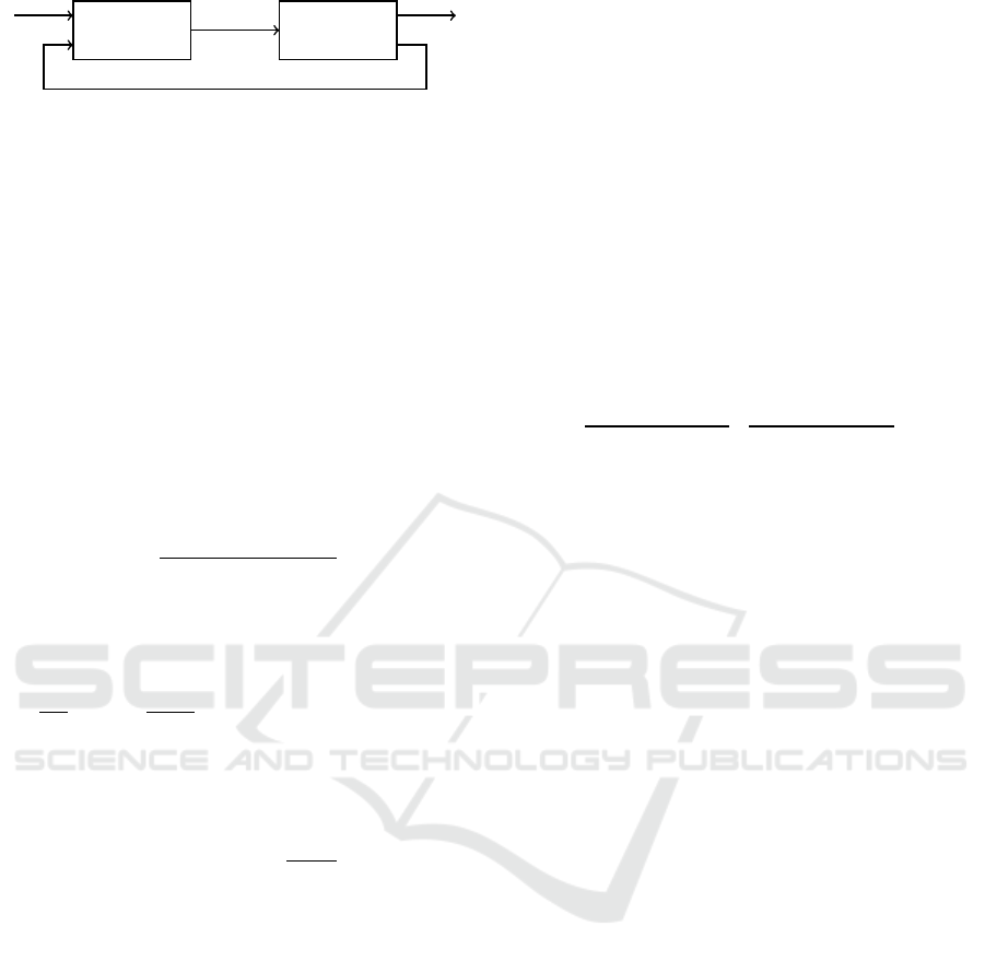
tem description is impossible because of curse of di-

mensionality. A system of order 100 has got more

than 10

terms in full representation, which does not

ﬁt in memory anymore. The state space representa-

tion and thus the computation of a controller of such

big system is not possible in a symbolical way.

Tensor decomposition methods like CP decomposi-

tion allow to compute low rank approximations of the

parameter tensors. This breaks the curse of dimen-

sionality and allows an approximate representation of

large scale systems with a number of parameters that

is lower by orders of magnitude. Figure 3 shows in

a logarithmic scale how the number of parameters in-

creases with the order of the system and the rank of

the parameter tensors.

Using low rank approximation techniques for pa-

rameter tensors, makes it possible to represent large

Figure 3: Number of parameter for MTI systems.

systems and to compute controllers as shown in this

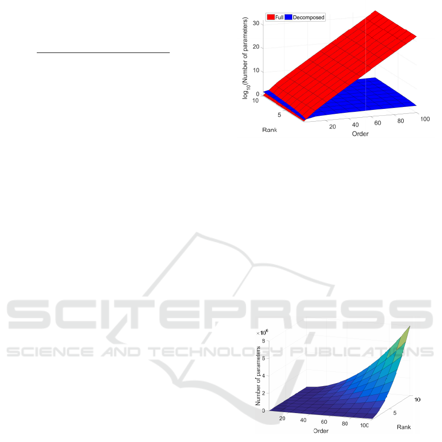
paper. E.g. the number of values to be stored for a

system of order 100 is reduced from 10

to 6200 for

a rank 10 approximation, since the parameters scale

linearly with order and rank. The proposed feedback

linearization approach works with the decomposed

representations of the system and all operations are

deﬁned for CP decomposed tensors such that no full

tensor representation has to be constructed during the

whole controller design process leading to a controller

in a decomposed structure. The storage demand is

still capable as shown in Figure 4, where an upper

bound for the number of elements to be stored for the

parameter tensors of the controller are depicted.

Figure 4: Upper bound for number of parameters for a feed-

back linearizing controller of decomposed MTI systems.

The ﬁgure considers different orders and different

ranks of the system tensors A, B and C for a sys-

tem with relative degree of one. Often the results

can be represented by tensors of lower rank which

reduces the storage effort further. Also during appli-

cation the controller law can be evaluated based on

the decomposed factor matrices. This makes it pos-

sible to use this feedback linearizing scheme also for

large scale MTI systems, where the full representa-

tion can not processed but low rank approximations

exist. This break of the dimensionality problem for

large scale systems is the big advantage of the intro-

duced feedback linearization design approach by CP

decomposed tensors.

Feedback Linearization of Multilinear Time-invariant Systems using Tensor Decomposition Methods

239

8 APPLICATION

In this section the proposed method for feedback lin-

earization is applied ﬁrst to a SISO, MTI system

with 2 states for giving all steps of the design pro-

cedure explicitly. Consider the system



˙x





−x

+ 0.2x







y = 1 + 2x

The systems belongs to the class of input afﬁne MTI

systems (47) and (48) where the factor matrices are

represented as CP tensors

A =



0 1 0

1 0 1





1 0 0

0 1 1





1 0 0

0 1 1







−1

0.2





B =













· 1,

C =



1 1

0 0





0 1

1 0







To design the controller, the Lie derivatives of the sys-

tem must be derived. Using (49) the parameter tensors

of the Lie derivatives along a(x) in CP representation

are given by

A,C,1

















· 4,

A,C,2



1 0

0 1





0 0

1 1





1 1

0 0



, ···



1 1

0 0





1 1

0 0





1 1

0 0





−4

0.8



resulting in the derivatives

c(x) =



A,C,1





= 4x

c(x) =



A,C,2





= −4x

+ 0.8x

The Lie derivatives along b(x) leads to L

c(x) = 0

and L

c(x) = 4 by the parameter tensors (50)

B,A,C,0

















· 0,

B,A,C,1

























· 4.

Because of L

c(x) = 4 6= 0 ∀x the relative degree ρ

of the system is two, which is equal to the number of

states. Thus the system has full degree and the zero

dynamics needs not to be checked. Additionally the

system is controllable and observable. In closed loop,

the linear behavior

¨y + µ

˙y + µ

y = µ

is desired. As an example µ

= µ

= 10 and µ

= 1

are chosen. Using the parameter tensors of the

Lie derivatives, the feedback linearizing controller is

given by

−



C+µ

A,C,1

+µ

A,C,2



(x)



+ µ



B,A,C,1



(x)



=−

10 + 16x

+ 40x

+ 0.8x

+ 10r

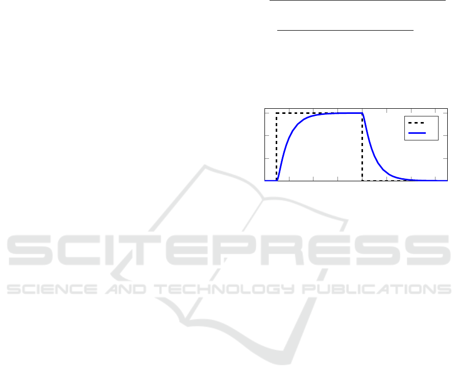
Figure 5 shows the closed loop simulation result

with x



−0.5 0



for a step change in reference

signal r. The system behaves as the speciﬁed 2

or-

der linear system.

0 2 4

8 10 12 14

Time [s]

Figure 5: Closed loop simulation.

9 CONCLUSION AND OUTLOOK

In this paper a feedback linearization approach for

CP decomposed MTI systems was derived. The con-

troller is determined numerically without any sym-

bolic computation. Therefore multiplication and dif-

ferentiation of polynomial functions are investigated

that are necessary for computation of the Lie deriva-

tives of the system. It is shown that the parameter ten-

sors of the result of these operations can be computed

efﬁciently by the parameter tensors of the operands if

in CP. With that the controller law of the feedback lin-

earizing controller is computed. This is an important

advantage when focusing large systems where a stan-

dard representation of right hand sides is not possible,

since the use of decomposition techniques leads to a

signiﬁcant reduction in storage demand by orders of

magnitude. This construction of the linearizing feed-

back gain leads to a controller with a structure that is

independent of the plant. Only a parameter set has to

be computed to use the controller for a special appli-

cation.

Here the standard method of feedback lineariza-

tion for SISO systems is investigated. This approach

could be extended to MIMO systems. From a math-

ematical point of view it is interesting to use other

tensor decomposition techniques for the design algo-

rithm like Tensor Trains, (Oseledets, 2011). Another

SIMULTECH 2018 - 8th International Conference on Simulation and Modeling Methodologies, Technologies and Applications

240

interesting point is to compare the proposed method

to other approaches of feedback linearization to de-

termine a threshold for the system size, where other

methods fail and the tensor methods is the only appli-

cable algorithm.

ACKNOWLEDGEMENTS

This work was partly sponsored by the project OB-

SERVE of the Federal Ministry of Economic Affairs

and Energy, Germany (Grant No.: 03ET1225B).

REFERENCES

Bader, B. W., Kolda, T. G., et al. (2015). Matlab tensor

toolbox version 2.6. Available online.

Cichocki, A., Mandic, D. P., Phan, A. H., Caiafa, C. F.,

Zhou, G., Zhao, Q., and Lathauwer, L. D. (2014).

Tensor decompositions for signal processing applica-

tions from two-way to multiway component analysis.

CoRR, abs/1403.4462.

Cichocki, A., Zdunek, R., Phan, A., and Amari, S. (2009).

Nonnegative matrix and tensor factorizations. Wiley,

Chichester.

Deutscher, J. (2005). Input-output linearization of nonlin-

ear systems using multivariable legendre polynomials.

Automatica, 41:299–304.

Ekman, M. (2005). Modeling and Control of Bilinear Sys-

tems: Application to the Activated Sludge Process.

PhD thesis, Uppsala University.

Grasedyk, L., Kressner, L., and Tobler, C. (2013). A lit-

erature survey of low-rank tensor approximation tech-

niques. GAMM-Mitteilungen, 36:53–78.

Hackbusch, W. (2012). Tensor Spaces and Numerical Ten-

sor Calculus, volume 42 of Springer Series in Com-

putational Mathematics. Springer-Verlag Berlin Hei-

delberg.

Isidori, A. (1995). Nonlinear Control Systems. Springer-

Verlag New York, Inc., Secaucus, NJ, USA, 3rd edi-

tion.

Khalil, K. H. (1996). Nonlinear Systems. Prentice-Hall,

Inc.

Kolda, T. and Bader, B. (2009). Tensor decompositions and

applications. SIAM Review, 51(3):455–500.

Kruppa, K. and Lichtenberg, G. (2016). Comparison of cp

tensors, tucker tensors and tensor trains for represen-

tation of right hand sides of ordinary differential equa-

tions. In Workshop on Tensor Decomposition and Ap-

plications, Leuven.

Kruppa, K., Pangalos, G., and Lichtenberg, G. (2014). Mul-

tilinear approximation of nonlinear state space mod-

els. In 19th IFAC World Congress, Cape Town, pages

9474–9479. IFAC.

Lichtenberg, G. (2010). Tensor representation of boolean

functions and zhegalkin polynomials. In International

Workshop on Tensor Decompositions, Bari.

uller, B. and Deutscher, J. (2005). Approximate input-

output linearization using l2-optimal bilinearization.

In Proceedings of the 44th IEEE Conference on De-

cision and Control and the European Control Confer-

ence.

uller, T., Kruppa, K., Lichtenberg, G., and R

ehault,

N. (2015). Fault detection with qualitative models

reduced by tensor decomposition methods. IFAC-

PapersOnLine, 48(21):416 – 421. 9th IFAC Sympo-

sium on Fault Detection, Supervision and Safety for

Technical Processes, SAFEPROCESS.

Oseledets, I. (2011). Tensor-train decomposition. SIAM

Journal of Scientiﬁc Computing, 33(5):2295–2317.

Pangalos, G. (2016). Model-based controller design meth-

ods for heating systems. Dissertation, TU Hamburg,

Hamburg.

Pangalos, G., Eichler, A., and Lichtenberg, G. (2015). Hy-

brid Multilinear Modeling and Applications, pages

71–85. Springer International Publishing, Cham.

obenack, K. (2005). Automatic differentiation and non-

linear controller design by exact linearization. Future

Generation Computer Systems, 21:1372–1379.

Vervliet, N., Debals, O., Sorber, L., Van Barel, M., and

De Lathauwer, L. (2016). Tensorlab 3.0. Available

online.

APPENDIX

In the Appendix the proofs of the arithmetic oper-

ations, i.e. multiplication, differentiation and Lie

derivative, for polynomials in tensor representation is

given. Furthermore, the proofs of th eouter product of

CP tensors and the control law for the feedback lin-

earizing controller for CP decomposed MTI systems

are presented here.

Proof of the Outer Product

Proof 1. Inserting the elementwise descriptions of X

and Y into the outer product (2), leads to

z(i

, . . . , i

, j

, . . . , j

) = x(i

, . . . , i

)y( j

, . . . , j

)

∑

k=1

(k)u

, k)···u

, k)

∑

k=1

(k)v

( j

, k)···v

( j

, k)

=λ

(1)λ

(1)u

,1)·· ·u

,1)v

( j

,1)·· ·v

( j

,1)

+λ

(1)λ

(2)u

,1)·· ·u

,1)v

( j

,2)·· ·v

( j

,2)

+ ··· + λ

)λ

, r

)· ·· v

( j

, r

Comparing this representation of the outer product

with the elementwise description of the resulting ten-

Feedback Linearization of Multilinear Time-invariant Systems using Tensor Decomposition Methods

241

sor in CP decomposition

z(i

, . . . , j

) =

∑

k=1

(k)w

, k)···w

n+m

( j

, k),

leads to the factors in (12) to (14).

Proof of the Multiplication

Proof 2. Considering (35) the monomial tensor of the

result can be decomposed by



◦H



(x)





◦H



(x) ◦M

(x)



Using the elementwise representations (2) and (4) of

outer and contracted product and rearranging gives



◦ H



(x) ◦ M

(x)



∑

·· ·

∑

·· ·

∑

, . . . , i

( j

, . . . , j

)

· m

(x)(i

, . . . , i

(x)( j

, . . . , j

)

∑

·· ·

∑

, . . . , i

(x)(i

, . . . , i

)

∑

·· ·

∑

( j

, . . . , j

(x)( j

, . . . , j

)





(x)







(x)



= h

(x) · h

(x)

Proof of the Differentiation

Proof 3. All terms depending on the variables x

with i = 1, . . . , n of a polynomial in tensor form are

inside the monomial tensor. The parameter tensor H

contains constant elements only. Thus, the partial

derivative of the monomial tensor is investigated ﬁrst.

In the multilinear case the partial derivative with re-

spect to one variable x

can be found using the prod-

uct rule of differentiation as stated in Proposition 1

∂

∂x

M(x)= [w

, . . . , w

] =

∂

∂x





◦ ··· ◦









◦·· ·◦



j+1



◦





◦



j−1



◦·· ·◦





. (52)

The factor matrices of the derivative of the monomial

tensor reads









0 1



, for i = n − j + 1,



1 x

n−i+1



, else.

The differentiation inﬂuences the dimension belong-

ing to the differentiation variable x

of the monomial

tensor only. Thus, the differentiation can be expressed

in terms of a k-mode product

∂

∂x

M(x) = M(x) ×

n− j+1

setting the factor matrix of M(x) belonging x



0 1



Since the partial derivative can be found for the mul-

tilinear monomial tensor, the concept is extended to

polynomials with higher monomial orders N ≥ 1. In

contrast to the multilinear case, the variable x

does

not occur in one factor matrix only but in N factor ma-

trices. According to the product rule of differentiation

the differentiation of M

(x) leads to

∂

∂x

(x) =

∑

k=1

, . . . , w

with









0 1



, for i = nk − j + 1,



1 x

nk−i+1



, else.

As before, this change in the factor matrices can be

expressed by k-mode product leading to the partial

derivative of the monomial tensor

∂

∂x

(x) =

∑

k=1

(x) ×

kn− j+1

. (53)

With the derivative of the monomial tensor (53) the

derivative of the function is given by

∂

∂x





(x)





∑

k=1

(x) ×

kn− j+1





(x)



. (54)

To ﬁnd the parameter tensor H

, (54) can be written



∑

k=1

(x) ×

kn− j+1

= (55)

∑

k=1





(x) ×

kn− j+1



because of the linearity property of the inner product.

The elements of the k-mode product read



(x) ×



, . . . , l, . . . , i

)

= m

, . . . , 1, . . . , i

)Θ

(l, 1),

because Θ

(l, 2) = 0, l = 1, 2. With that, the terms of

the sum in (55) are written as





(x) ×



∑

·· ·

∑

h(i

, . . . , i

, . . . ,1, . . . , i

)Θ

(l,1).

SIMULTECH 2018 - 8th International Conference on Simulation and Modeling Methodologies, Technologies and Applications

242

The aim is to isolate the monomial tensor on the right

side of the contracted product such that





(x) ×







(x)



∑

·· ·

∑

h(i

, . . . , i

Therefore, the elements of

H are given by

h(i

, . . . ,i

, . . . , i

(

h(i

, . . . ,2, . . . ,i

), for i

=1,

0 , for i

=2,

since

∑

h(i

, . . . ,i

)Θ

(l,1) = h(i

, . . . ,2, . . . , i

Using Deﬁnition 4 of the k-mode product, the param-

eter tensor

H can be directly computed by

H = H ×

Θ,

leading to





(x) ×





H ×



(x)



Inserting this to (55) shows that the partial derivative

of a polynomial h(x) is computed by

∂

∂x





(x)



∑

k=1



H ×

kn− j+1



(x)



∑

k=1

H ×

kn− j+1



(x)

such that the parameter tensor of the derivative reads

∑

k=1

H ×

kn− j+1

Θ.

Proof of the Lie Derivative

Proof 4. The ﬁrst Lie derivative, i.e. l = 1, of g(x)

along h(x) is deﬁned by

g(x) =

∑

i=1

(x)

∂

∂x

g(x). (56)

Since the scalar function g(x) is given as tensor func-

tion, equation (41) is applied to get the partial deriva-

tive

∂

∂x

g(x) =

∑

k=1

G×

kn−i+1



(x)

, i =1, . . . , n.

The multiplication with h

(x) =





(x)



where i = 1, . . . , n using (38) yields

(x)

∂

∂x

g(x) =

◦

∑

k=1

G×

kn−i+1



(x)

Summing up these elements to get the Lie deriva-

tive (56) leads to

g(x) =

∑

i=1

◦

∑

k=1

G×

kn−i+1



(x)

∑

i=1

◦

∑

k=1

G×

kn−i+1



(x)

This approach is extended to multiple Lie derivatives

along h(x) as given by (45) for arbitrary l ∈ N by

g(x) =

∑

i=1

(x)

∂

∂x

l−1

g(x)

∑

i=1





(x)



∑

k=1

H,G,l−1

kn−i+1



(x)

∑

i=1

◦

∑

k=1

H,G,l−1

kn−i+1



(l+1)N

(x)

Proof of the Feedback Linearizing

Controller

Proof 5. Inserting the tensor representation of the

Lie derivatives deﬁned in Lemma 1 into the controller

function (30) and rearranging leads to

−

∑

i=0



A,C,i



i+1

(x)



+ µ

B,A,C,ρ−1



ρ+1

(x)

−



∑

i=0

A,C,i



ρ+1

(x)



+ µ

B,A,C,ρ−1



ρ+1

(x)

Feedback Linearization of Multilinear Time-invariant Systems using Tensor Decomposition Methods

243