State Feedback Optimal Control with Singular Solution

for a Class of Nonlinear Dynamics

Paolo Di Giamberardino

and Daniela Iacoviello

1,2

Dept. Computer, Control and Management Engineering Antonio Ruberti, Sapienza University of Rome, Italy

Institute for Systems Analysis and Computer Science Antonio Ruberti, Rome, Italy

Keywords:

Optimal Control, Singular Control, Costate Independent Singular Surface, SIR Epidemic Model.

Abstract:

The paper studies the problem of determining the optimal control when singular arcs are present in the solution.

In the general classical approach the expressions obtained depend on the state and the costate variables at the

same time, so requiring a forward-backward integration for the computation of the control. In this paper,

sufﬁcient conditions on the dynamics structure are provided and discussed in order to have both the control

and the switching function depending on the state only, so simplifying the computation avoiding the necessity

of the backward integration. The approach has been validated on a classical SIR epidemic model.

1 INTRODUCTION

Optimal control theory provides the natural frame-

work to solve control problems when contrasting go-

als are required with resource limitations. The de-

sign procedure can make use of the minimum princi-

ple, allowing the determination of the optimal cont-

rol that, depending on the cost index and on the mo-

deling, could be a bang-bang or a bang-singular-bang

solution, (Athans and Falb, 1996; Hartl et al., 1995;

Johnson and Gibson, 1963; Bryson and Ho, 1969).

In particular, if the model as well as the cost index

are linear in the control, the existence conditions of

such kind of solutions can be explicitly determined.

In the bang-bang solution the control assumes only

the extreme values, whereas the singular one is obtai-

ned if the Hamiltonian does not depend on the control

in an interval of positive measure. The extreme va-

lues assumed by the control depend on the sign of the

switching function, whereas the existence of singu-

lar control is related to the possibility that this swit-

ching function is identically zero on an interval of ﬁ-

nite length.

The determination of singular control, while it is

easy from a theoretical point of view, is generally dif-

ﬁcult to implement; the optimal control requires the

solution of a non linear differential equations system

in the state variables with initial conditions, and a non

linear differential equations system in the costate va-

riables with ﬁnal conditions. Moreover, in general it

is not easy the determination of the best control se-

quence and the number of switching points, (Vossen,

2010; Fraser-Andrews, 1989).

In this paper, the determination of the optimal con-

trol of nonlinear systems is investigated referring to

the case in which the input acts linearly both in the

model and in the cost index, aiming at a constructive

computing of the singular solution. This approach

is then applied to a classical SIR epidemic problem,

where S stands for the class of susceptible subjects, I

for the class of infected patients and R for the class of

the removed ones (Di Giamberardino and Iacoviello,

2017; Bakare et al., 2014). Optimal control for epi-

demic spread containment has been widely used in

literature (Behncke, 2000; Di Giamberardino et al.,

2018). In particular, the optimal singular control for a

SIR epidemic model has been already studied in (Le-

dzewicz and Schattler, 2011; Ledzewicz et al., 2016),

where the structure of singular control has been dee-

ply investigated in presence of the double control,

vaccination and medical treatment, showing that the

latter can’t be singular, whereas a singular regimen is

expected for the optimal vaccination strategy. Diffe-

rently from (Ledzewicz et al., 2016), in this paper a

recovered subject could neither become susceptible,

nor infected again. Therefore, it is possible to study

the singular surface, that is the manifold over which

the state variables move under the action of the singu-

lar control, if it exists. Facing epidemic spread cont-

rol in the framework of optimal control theory is rat-

her common for its capability of suggesting suitable

scheduling of possible actions such as vaccination or

336

Giamberardino, P. and Iacoviello, D.

State Feedback Optimal Control with Singular Solution for a Class of Nonlinear Dynamics.

DOI: 10.5220/0006859903360343

In Proceedings of the 15th International Conference on Informatics in Control, Automation and Robotics (ICINCO 2018) - Volume 1, pages 336-343

ISBN: 978-989-758-321-6

quarantine or treatment, taking into account resource

limitations. The paper is organized as follows; the

optimal control problem is formulated in Section 2,

describing the conditions and the constraints usually

considered and giving the structure of the optimal so-

lution as well as the conditions for the existence of

both switches and singular arcs. Then, in Section 3

the class of dynamics considered is introduced and

constructive conditions for the singular solutions are

given for different formulations of the optimal pro-

blem. In Section 4 the case study describing the SIR

epidemic spread is introduced to verify and highlight

the effectiveness of the results.

2 THE OPTIMAL CONTROL

PROBLEM FORMULATION

The optimal control problem here addressed is refer-

red to the design of the control input u, for a given

nonlinear dynamics of the form

˙x = f (x) + g(x)u = f (x) +

∑

i=1

(x) (1)

where x ∈ R

, u ∈ R

and with x(t

) = x

, such that a

cost index

J =

L(x, u,t)dt (2)

L : R

× R

× R → R, is minimised.

Usually, a bound on the input amplitude is consi-

dered, so that the control must satisfy

min

≤ u(t) ≤ u

MAX

∀t ∈ [t

] (3)

with u

min

, u

MAX

∈ R

In the deﬁnition of the problem, additional con-

straints can be introduced.

i. The ﬁnal time instant t

can be ﬁxed, so that the

cost index results to be a function of the input only

J(u) =

L(x, u,t)dt (4)

Be t

such a preﬁxed value, a constraint of the

form

χ(x(t

),t

) = 0 (5)

with χ(t

) = t

− t

has to be considered, with

χ ∈ C

almost everywhere, dim

{

}

= 1.

ii. The ﬁnal value for the state x(t

) = x

, or for σ

components only, can be ﬁxed; in this case, x(t

)

must satisfy a condition of the form χ (x(t

)) =

x(t

) − x

, with dim

{

}

= σ, 1 ≤ σ ≤ n, and the

cost index is a function of both u and t

J(u, t

) =

L(x, u,t)dt (6)

Clearly, if t

is left free, it has to be found along

the solution computation.

The usual design procedure starts with the deﬁni-

tion of the Hamiltonian function

H(x, λ, u, t) = L(x, u, t) + λ

( f (x) + g(x)u) (7)

in which the multiplier function λ(t) is introduced,

with λ(t) : R → R

, λ(t) ∈ C

almost everywhere.

The Hamiltonian (7) veriﬁes the condition

H(x, λ, u, t) = K ∀t ∈ [t

] (8)

with K ∈ R. Since (7) must satisfy

H(x, λ, u, t

) =

∂χ(x(t

),t

)

∂t

η (9)

for an unknown η ∈ R, K is a variable to be found

during the optimization procedure if the ﬁnal time t

is ﬁxed, with K = η, as in the previously mentioned

case i., while it is equal to zero when the ﬁnal time is

left free.

From (7), and taking into account the dynamics

form (1), the differential equation describing the be-

haviour of λ can be obtained as

λ = −

∂L

∂x



−

∂ f

∂x



∑

i=1

∂g

∂x



under the boundary conditions

λ(t

) = −

∂χ(x(t

),t

)

∂x(t

)



ζ (10)

with ζ ∈ R

to be found and χ in (5). Clearly, if con-

straint (5) is not present, (10) becomes

λ(t

) = 0 (11)

The structure of (7) suggests that if in L(x, u, t)

the control u is present with a linear contribution, the

whole Hamiltonian results to be afﬁne with respect to

the control. This property can be very useful when the

minimum principle is applied.

Then, particularising the expression

L(x, u,t) =

L(x,t) + c

u (12)

the structure of L as in (12), used in (7), gives the

compact expression

H(x, λ, u, t) =

L(x,t) + c

u + λ

f (x) + λ

g(x)u =

L(x,t) + λ

f (x) +



+ λ

g(x)



u =

= F(x, λ, t) + G(x, λ)u (13)

with

F(x, λ, t) =

L(x,t) + λ

f (x) (14)

G(x, λ) = c

+ λ

g(x) (15)

State Feedback Optimal Control with Singular Solution for a Class of Nonlinear Dynamics

337

Clearly, the presence of the input u in the cost

function in a linear form is always possible, if u

min

in (3) is ﬁnite.

The minimum principle H(x, λ, u, t) ≤

H(x, λ, ω, t) ∀ω ∈ [u

min

, u

MAX

] can be used, gi-

ving, for (13), the condition G(x, λ)u ≤ G(x, λ)ω

∀ω ∈ [u

min

, u

MAX

]. As a consequence, the optimal

control

u =



MAX

if G(x, λ) < 0

min

if G(x, λ) > 0

(16)

can be obtained. The time instant t

such that

G(x(t

), λ(t

)) = 0 (17)

with

G(x

−

), λ

−

)) G(x

), λ

)) < 0

is the instant of switching in which the control chan-

ges from one extreme to the other, so getting a classi-

cal bang-bang solution. If condition (17) holds over a

ﬁnite time interval

G(x

(t), λ

(t)) = 0 t

≤ t

≤ t ≤ t

≤ t

(18)

with t

> t

, then the optimal control presents a sin-

gular solution and it assumes the form

u =







MAX

if G(x, λ) < 0

, λ

) if G(x, λ) = 0

min

if G(x, λ) > 0

(19)

In this case, (18) means that G(x(t), λ(t)) is con-

stant over a ﬁnite time interval and, then, the identities

∂

G(x(t), λ(t))

∂t

= G

(k)

(x(t), λ(t)) = 0 ∀t ∈ [t

]

(20)

must hold for any k ≥ 0. Computing (20), for

k = 0, 1, 2, . . . , there exists an index r such that

(k)

(t), λ

(t)) is independent from u if k < r,

while, for k = r, the control u appears explicitly.

Then, the ﬁrst r conditions (20), for k = 0, . . . , r − 1,

give r relations between state x and costate λ, and

from G

(r)

(x(t), λ(t)) = 0 the expression for the sin-

gular control u

in (19) can be obtained.

Making reference to the expression (15), one has

(0)

(x, λ) = c

+ λ

g(x) = 0 (21)

(1)

(x, λ) =

g(x) + λ

˙g(x) =

= −α

g(x) − λ

f (x) −

∑

i=1

(x) +

+λ

g(x) +

∑

i=1

g(x) =

= −α

g(x) + λ

g(x) +

∑

i=1

g(x) = 0 (22)

where the compact expressions

g(x) = (L

(x). . . L

(x)) (23)

f (x) = (L

f (x) . . . L

f (x)) (24)

(x) = (L

(x) . . . L

(x)) (25)

g(x) = (L

(x) . . . L

(x)) (26)

g(x) = L

g(x) − L

f (x) (27)

g(x) = L

g(x) − L

(x) (28)

are used. Note that the structures of the Lie Bracket

introduced are

g(x) =



(x) ad

(x) ··· ad

(x)



g(x) =



(x) ad

(x) ··· ad

(x)



recalling that ad

(x) = 0 ∀i ∈ [1, m].

If dynamics (1) is such that the vector ﬁelds g

commute, then

∑

i=1

g(x) = 0, as in (Ledze-

wicz and Schattler, 2011; Ledzewicz et al., 2016); the

identity (22) reduces to

(1)

(x, λ) = −α

g + λ

g(x) = 0 (29)

and G

(2)

(x, λ) has to be computed, iterating the pro-

cedure. As well known (Bryson and Ho, 1969), this

iteration ends at a ﬁnite index r such that G

(r−1)

(x, λ)

is not dependent from u while G

(r)

(x, λ) is, so giving

the control expression as a function of the x and λ.

3 BLOCK SUB TRIANGULAR

SINGLE INPUT SYSTEMS

The class of dynamics (1) considered is here particu-

larised setting x non negative and m = 1. Such choi-

ces allow to simplify the notations: m = 1 gives a

simpler expression for the input contribution from (1)

on, while, thanks to the non negativeness of the state,

L(x,t) = α

x can be used, so obtaining a fully linear

term in the cost function. Then,

λ in (10) becomes

λ = −α −

∂ f

∂x



λ − u

∂g

∂x



λ (30)

while the existence of singular solutions gives for the

conditions (21) and (22) on the G

(k)

(t), λ

(t)) the

expressions

(0)

(x, λ) = c + λ

g(x) = 0 (31)

(1)

(x, λ) = −α

g(x) + λ

g(x) = 0 (32)

ICINCO 2018 - 15th International Conference on Informatics in Control, Automation and Robotics

338

with (32) always independent from u. Then, also the

computation of G

(2)

(x, λ, u) = 0 must be performed:

(2)

(x, λ, u) = −α

g(x) + uL

g(x)) +

−



+ λ

∂ f

∂x

+ uλ

∂g

∂x



g(x) +

+λ

g(x) + uL

g(x)) =



g(x) − α

g(x) + ad

g(x))



−



g(x) − λ

g(x)



u (33)

If α

g(x) − λ

g(x) 6= 0, the singular

control u

can be obtained as

(x, λ) =

g(x) − α

g(x) + ad

g(x))

g(x) − λ

g(x)

(34)

otherwise G

(2)

(x, λ, u) = G

(2)

(x, λ), the condition

g(x) − α

g(x) + ad

g(x)) = 0 (35)

involving x and λ only, is obtained, and a further de-

rivative G

(3)

(x, λ, u) must be computed. Set r as the

ﬁrst index such that G

(r)

(x, λ, u) is dependent from the

input. It is easily veriﬁed that

Proposition 1. The expression of the i–th derivative

(i)

(x, λ), for i = 0, 1, . . . , r − 1, is of the form

(i)

(x, λ) = λ

g(x) + h

(x)

for suitable functions h

(x) (h

(x) = c, h

(x) =

−α

g(x)).

Proof: It comes iteratively at i–th step from the struc-

ture of G

(i−1)

(x, λ) and the computations evidenced in

(33).

The class of nonlinear dynamics considered is of

the form



˙x





)





)



u (36)

where x

∈ R

, x

∈ R

n−r

, and the functions f

and g

deﬁned consequently. The controllability condition

dim



span

, ad

, . . . , ad

r−1

)



= r (37)

for the ﬁrst subsystem is assumed veriﬁed, with x

in a suitable domain containing x

). The example

used in Section 4 to illustrate the proposed approaches

fulﬁls this hypothesis with r = 2.

Consequently, setting

λ =





∈ R

, λ

∈ R

n−r

(38)

one has

∂L

∂x



∂L

∂x

∂L

∂x



∂ f

∂x

∂ f

)

∂x

∂ f

)

∂x

∂g

∂x

∂g

)

∂x

∂g

)

∂x

so that (10) becomes





= −

∂L

∂x

∂L

∂x

∂ f

)

∂x

∂ f

)

∂x

0 0

λ +

∂g

)

∂x

∂g

)

∂x

0 0

λ (39)

The above equation can be explicitly decomposed

into

= −

∂L

∂x

−



∂ f

)

∂x

+ u

∂g

)

∂x



−



∂ f

)

∂x

+ u

∂g

)

∂x



(40)

= −

∂L

∂x

(41)

From this structure, and on the basis of the expres-

sion of constraint (5), if present, one has the following

proposition:

Proposition 2. Given the optimal control problem,

with ﬁxed time t

and free ﬁnal conditions on the state,

for a non linear dynamics of the form (36) and the

cost function (4) with L(x, u, t) = α

+ cu, α

∈ R

there exists an algorithm for the computation of the

optimal singular solution which gives the expression

of the control law as a pure state feedback, bringing to

a bang–singular–bang optimal control, for which the

singular surface can be explicitly written as a state

function only. Moreover, after the last switch, the op-

timal control u is equal to u

min

Proof: The independence of the constraint (5) from

the state x(t

) makes (11) hold; moreover, the choice

for L(x, u, t) gives, for equation (41), the simple ex-

pression

= 0 which, for (11) and for the continuity

hypothesis on λ(t), gives λ

(t) = 0 ∀t ∈ [t

]. This

means that, for t = t

, G(x, λ) = c ≥ 0, and then the

last condition in (19) is satisﬁed. Moreover, for the

continuity conditions on x and λ, the inequality must

hold over a ﬁnite time interval, which necessarily cor-

responds to the last bang interval, so proving the last

claim of the Proposition.

Equations G

(i)

(x, λ), i = 0, 1, . . . , r − 1, can be re-

State Feedback Optimal Control with Singular Solution for a Class of Nonlinear Dynamics

339

written as

(0)

(x, λ) = λ

) + c = 0 (42)

(1)

(x, λ) = λ

) − α

) = 0

(43)

. . . = . . .

(r−1)

(x, λ) = λ

r−1

) + h

r−1

) = 0

(44)

or in the compact form



), ad

), . . . ad

i−1

)





−c, α

), . . . h

i−1

)



from which

= (−c, . . . h

i−1

))



), . . . ad

i−1

)



−1

(45)

can be computed under the controllability condition

(37). Then, the costate λ is fully known, at least as a

function of the state. A ﬁrst consequence of this fact is

the possibility to express the singular control u

(x, λ)

as a state function only, in particular a function of x

= u

Now, from (8), applied in (13) and then in (14)

when (18) holds, one gets the expression

F(x, λ, t) = α

+ λ

) = K (46)

which, using (45), brings to the state function

K = α

+(−c . . . h

i−1

))



) . . . ad

i−1

)



−1

)

(47)

which fully describes the singular surface in the x

subspace. As far as the subspace x

is concerned,

once the evolution of x

is determined, also x

is fully

known, since (36), the singular control u

) and the

evolution of x

satisfying (47) allow to compute x

(t)

∀t ∈ [t

]. The value of the unknown parameter K

can be computed noting that, from (13) evaluated af

t = t

, one has

H(x, λ, u, t

) = α

) = K (48)

being u(t

) = 0 as well as λ(t

) = 0. Expression (48),

once x(t

) is computed, gives K.

Proposition 2 allows to fully compute the singular

part of the optimal solution. The full solution (19) is

obtained including the conditions in (16).

Proposition 3. Given the optimal control problem,

with ﬁxed time t

and ﬁxed ﬁnal condition on the state

x(t

) = x

, for a non linear dynamics of the form (36)

and the cost function (4) with L(x, u,t) = α

+ cu,

∈ R

, there exists an algorithm for the computa-

tion of the optimal singular solution which gives the

expression of the control law as a pure state feed-

back, bringing to a bang–singular–bang optimal con-

trol, for which the singular surface can be explicitly

written as a state function only.

Proof: The presence of constraint (5) does not allow

to know λ(t

) due to expression (10). However,

0 is still true and then one has λ

(t) = λ

) = const.

In this case equations (42), (43), (44) assume the form

(0)

(x, λ) = λ

) + λ

) = 0 (49)

(1)

(x, λ) = λ

) − α

) +

+λ

)[ f

, g

](x

) = 0 (50)

. . . = . . .

(r−1)

(x, λ) = λ

r−1

) + h

r−1

(λ

), x

)

(51)

The same considerations as in the proof of Propo-

sition (2) can be carried on, computing λ

as in (45),

whose expression in this case is λ

(λ

), x

). Both

the singular control u

and the singular surface (47)

can be computed, as in the proof of Proposition 2,

as function of x

but they results to be parametrised

by λ

). The same follows for x

(t). However, the

imposition of condition (5) allows to determine the

actual values for λ

), so getting again the full com-

putation of the singular solution u

= u

) and of

the singular state space surface. The full knowledge

of all the state and control variables at t = t

allows to

obtain the value K from the evaluation of (13) at the

ﬁnal time, as for the previous Proposition.

The last case here addressed refers to a free time

ﬁxed ﬁnal conditions on the state variables. It is pos-

sible to state the following

Proposition 4. Given the optimal control problem,

with free ﬁnal time t

and the constraint (5) for the

ﬁnal conditions on the state, for a non linear dyna-

mics of the form (36) and the cost function (4) with

L(x, u,t) = α

+ cu, α

∈ R

, there exists an algo-

rithm for the computation of the optimal singular so-

lution which gives the expression of the control law as

a pure state feedback, bringing to a bang–singular–

bang optimal control, for which the singular surface

can be explicitly written as a state function only.

Proof: The proof comes straightforwardly from the

one of Proposition 3, since the only difference is in

the fact that being the ﬁnal time t

free, K in (8) and

in all the derived expressions, as far as (47), is equal

to zero. All the other considerations still hold.

The procedure is illustrated in next Section ma-

king reference to a classical SIR epidemic diffusion,

for which several optimal control approaches can be

found in literature.

ICINCO 2018 - 15th International Conference on Informatics in Control, Automation and Robotics

340

4 EXAMPLE

With reference to the general formulation introduced

in Section 2, it is now considered the classical mathe-

matical model describing the SIR epidemic spread

S = −βSI −Su + µ (52)

I = βSI − γI (53)

R = γI (54)

with given initial conditions S

, I

, R

, and box con-

straints u(t) ∈ [0, u

MAX

], for which the control law

u(t) minimising the cost function

J(S(t), I(t), R(t), u(t)) =

(aI(t) + cu(t))dt (55)

has to be found. t

is assumed ﬁxed. The aim of the

control action is to minimize the number of infected

subjects I in the ﬁxed time interval [0, t

] by using as

less resources as possible; the positive parameters a

and c represent the weights of these two contrasting

requirements.

Setting

x =





with x





and x

= R (56)

the formulation corresponds to the case considered

in Proposition 2, with r = 2, α



0 a



, α





and

) =



−βSI + µ

βSI − γI



) =



−S



) = γI g

) = 0

(57)

Introducing

λ =





with λ

∈ R

and λ

∈ R (58)

the Hamiltonian (13) can be written as

H(x, λ, u) = α

+ cu + λ

) + λ

) +

+λ

)u =

= α

+ λ

) + λ

) +



c + λ

)



u =

= F(x, λ) + G(x, λ)u (59)

with

F(x, λ) = α

+ λ

) + λ

) (60)

G(x, λ) = c + λ

) (61)

and for which

H(x, λ, u) = K ∀t ∈ [t

], K ∈ R (62)

The costate dynamics (40) and (41) for λ can be

computed, getting

= −





−



−βI βI

−βS βS − γ



−u



−1 0

0 0



−





(63)

= 0 (64)

with λ(t

) = 0 from the free ﬁnal state x condition.

Then, as expected, from (64) one has λ

(t) = 0.

The computation of ad

) yields

) =



βSI − µ



−



βSI

−βSI





−µ

βSI



(65)

so that expressions (49) and (50) assume the form

(0)

(x, λ) = c + λ



−S



= 0 (66)

(1)

(x, λ) = λ



−µ

βSI



= 0 (67)

from which the variable λ

can be computed, as a

function of x



S I



, obtaining



−S 0

−µ βSI



−1



−c





µc

βS



(68)

The expression for G

(2)

(x, λ) can be computed as

(2)

(x, λ) = λ

) − α

) +

+uλ

) (69)

from which the singular control

(x, λ) =

) − α

)

(70)

is obtained. Computing

) =



−βµI + β

−β

+ 2βµI



(71)

) =



−µ

−βSI



(72)

in (70), and making use of (68), the state feedback

singular control

(x) =

aβSI − β

cSI +

2βcµI

−

2cµ

−2

cµ

= βI



βc − a

2cµ

− 1



(73)

is computed. Then, the full state feedback control law

(19) is obtained.

State Feedback Optimal Control with Singular Solution for a Class of Nonlinear Dynamics

341

From (60), according to (46) and (47), one has for

the singular surface



0 a









µc

βS





−βSI + µ

βSI − γI



aI − βcI +2

cµ

−

cγµ

βS

= K (74)

Finally, from (48),

K = aI(t

) (75)

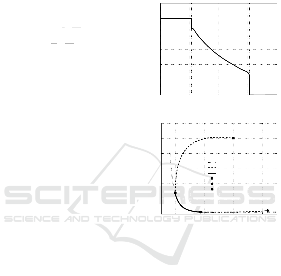
The time history of the bang-singular-bang control

is depicted in Figure 1, where the time instant t = 5.32

in which it switches from the constant value u

MAX

= 1

to u

, and the time t = 15.3, in which it switches from

min

= 0 are evidenced by the two vertical dotted

lines. The corresponding state evolution is represen-

ted in Figure 2 for the x

–x

plane projection: the ini-

tial part of the trajectory from the starting conditions

1,0

= 50 and x

2,0

= 10, the squared point, to the inter-

section with the singular curve (dotted line), denoted

by a dashed curve, represents the evolution under the

upper bound value for the control. Then, under the

singular control (73), the trajectory follows the singu-

lar curve along the solid arc, until the second switch

from u = u

to u = u

min

= 0 occurs, yielding to the

free evolution from the singular arc to the ﬁnal point

(diamond marker).

The simulation has been performed setting t

20, ﬁxing the model parameters to β = 0.01, γ = 0.4

and µ = 10 and choosing the weights α = 1 and c = 1

in the cost function (55).

5 CONCLUSIONS

Sufﬁcient conditions under which the solution of a

singular optimal control problem can be directly ex-

pressed as a state feedback law are provided, allowing

its computation by means of a simple forward integra-

tion of the system dynamics only. The class addressed

can be enriched, preserving the results, requiring the

introduction of some integrability properties for trian-

gular and sub triangular structure; this analysis is the

object of a forthcoming work.

ACKNOWLEDGEMENTS

This work was supported by Sapienza University

of Rome, Grants No. RP11715C82440B12 and

No. 191/2016.

0 5 10 15 20

0.2

0.4

0.6

0.8

Time t

u(t)

Figure 1: The Bang–Singular–Bang optimal control u(t).

0 10 20 30 40 50 60 70 80

(t)

Singular curve SC

State trajectory

Trajectory on the SC

Initial condition

Final condition

Switching points

Figure 2: State trajectory in the x

–x

plane, compared with

the singular curve.

REFERENCES

Athans, M. and Falb, P. (1996). Optimal Control. McGraw-

Hill, Inc., New York.

Bakare, E., Nwagwo, A., and Danso-Addo, E. (2014). Op-

timal control analyis of an sir epidemic model with

constant recruitment. International Journal of App-

lied Mathematical Research, 3.

Behncke, H. (2000). Optimal control of deterministic epi-

demics. Optimal control applications and methods,

21.

Bryson, A. and Ho, Y. (1969). Applied optimal control:

optimization, estimation, and control.

Di Giamberardino, P., Compagnucci, L., Giorgi, C. D., and

Iacoviello, D. (2018). Modeling the effects of pre-

vention and early diagnosis on hiv/aids infection dif-

fusion. IEEE Transactions on Systems, Man and Cy-

bernetics: Systems.

Di Giamberardino, P. and Iacoviello, D. (2017). Optimal

control of SIR epidemic model with state dependent

ICINCO 2018 - 15th International Conference on Informatics in Control, Automation and Robotics

342

switching cost index. Biomedical Signal Processing

and Control, 31.

Fraser-Andrews, G. (1989). Finding candidate singular op-

timal controls: a state of art survey. Journal of Opti-

mization Theory and Applications, 60.

Hartl, R., Sethi, S., and Vickson, R. (1995). A survey of

the maximum principles for optimal control problems

with state constraints. Society for Industrial and App-

lied Mathematics, 37:181–218.

Johnson, C. and Gibson, J. (1963). Singular solutions in

problems of optimal control. IEEE Trans. on Automa-

tic Control, 8(1):4–15.

Ledzewicz, U., Aghaee, M., and Schattler, H. (2016). Opti-

mal control for a sir epidemiological model withtime-

varying population. 2016 IEEE Conference on Cont-

rol Applications.

Ledzewicz, U. and Schattler, E. (2011). On optimal singu-

lar controls for a general SIR-model with vaccination

and treatment. Discrete and continuous dynamical sy-

stems.

Vossen, G. (2010). Switching time optimization for bang-

bang and singular controls. Journal of Optimization

Theory and Applications, 144.

State Feedback Optimal Control with Singular Solution for a Class of Nonlinear Dynamics

343