Quadcopter Control Approaches and Performance Analysis

Vasco Brito

1,2

, Alexandre Brito

, Luis Brito Palma

1,2

and Paulo Gil

1,2,3

Universidade Nova de Lisboa-FCT-DEE, 2829-516 Caparica, Portugal

Uninova-CTS, 2829-516 Caparica, Portugal

Universidade de Coimbra-CISUC, 3030-290 Coimbra, Portugal

Keywords:

Quadcopter Drone, Kinematic and Dynamic Models, PID Controller, Sliding Mode Controller, Faults and

Failures.

Abstract:

This article presents the kinematic and dynamic model of a X8 quadcopter, as well as control methodologies

based on the PID controller and Sliding Mode Controller. The main contributions are centered on the control-

lers tuning based on particle swarm optimization algorithm and on the controllers performance comparison

for nominal operation and for faulty situations. In order to show the overall performance, simulation results

for trajectory and orientation tracking control are presented.

1 INTRODUCTION

All aerial vehicles need to sustain a means to maintain

its body aloft, for that purpose several kinds of vehi-

cles were invented to tackle elevation in a comple-

tely different manner, for example the air balloon uses

temperature to levitate, the air plane uses the pressure

on the wings to glide and the helicopter uses the thrus-

ting force of the propellers to hover.

From the various types of aerial vehicles menti-

oned before, this paper’s content will ﬁt in the Ver-

tical Take-Off and Landing (VTOL) sort of aircraft.

The methodology for this aerial technology is quite

similar to the helicopter’s principle, in which both of

them hover by pushing the air downwards, (Luukko-

nen, 2011). The main difference relies on the number

of propellers and their respective placement and angle

allowing linear and angular movement, thereby gran-

ting them the same six degrees of freedom: North (x),

East (y), Down (z), Roll (φ), Pitch (θ) and Yaw (ψ).

In the world of Unmanned Aerial Vehicles (UAVs),

the quadcopter’s modelling and control are research

ﬁelds that have been particularly growing. The com-

mercial companies, military and even the tech com-

munity have been investing in these research ﬁelds,

(Merz and Kendoul, 2013). This piece of techno-

logy is currently used to facilitate tasks that are simple

enough for an unmanned drone to do, specially in the

entertainment, ﬁlming, surveillance and logistic sec-

tors (ie.:support on human rescue procedures, (TIME,

2015)). Although it looks simple to make a drone ho-

ver, move or even complete certain routes, it is not. It

has proven to be an extremely hard task to develop a

controller that could stabilize a quad-rotor during its

complex movements, since this system yields a very

fast dynamic behavior and is highly nonlinear.

A study of the most common controllers regarding

quacopter ﬂight was done here. In this work, the most

used kinds of control approaches were implemented

(PID (Mustapa et al., 2014) (Leong et al., 2012), Sli-

ding Mode (Bouabdallah and Siegwart, 2005) (Yih,

2016)), and their behavior regarding faults/failures

were evaluated.

A fault is an inconsistency happening in a running

dynamical system that deviates its optimal functi-

oning status but could compromise it as a whole

(Blanke et al., 2006). A failure is a permanent in-

terruption of a system’s ability to perform a required

function under speciﬁed operating conditions (Iser-

mann and Ball

e, 1997). In this research, a fault tole-

rant control approach was implemented, allowing the

prevention of a global system failure.

These controllers were implemented and tested on

a quadcopter model with two rotors on each arm anti-

parallel to each other and rotating in opposite directi-

ons. This eight rotor, four armed architecture is desig-

nated X8 quadcopter and is illustrated in Fig. 1 and

Fig. 2. As it will be explained further in this paper,

the main purpose of this architecture is to allow the

drone’s model, that happens to suffer a fault/failure in

sensors or actuators, to keep ﬂying and continue his

task. The X8 architecture does not bring efﬁciency

Brito, V., Brito, A., Palma, L. and Gil, P.

Quadcopter Control Approaches and Performance Analysis.

DOI: 10.5220/0006902600860093

In Proceedings of the 15th International Conference on Informatics in Control, Automation and Robotics (ICINCO 2018) - Volume 1, pages 86-93

ISBN: 978-989-758-321-6

battery wise but it does bring a lot more safety to

the aircraft’s structure, as well as acuators redundancy

(Brito et al., 2016).

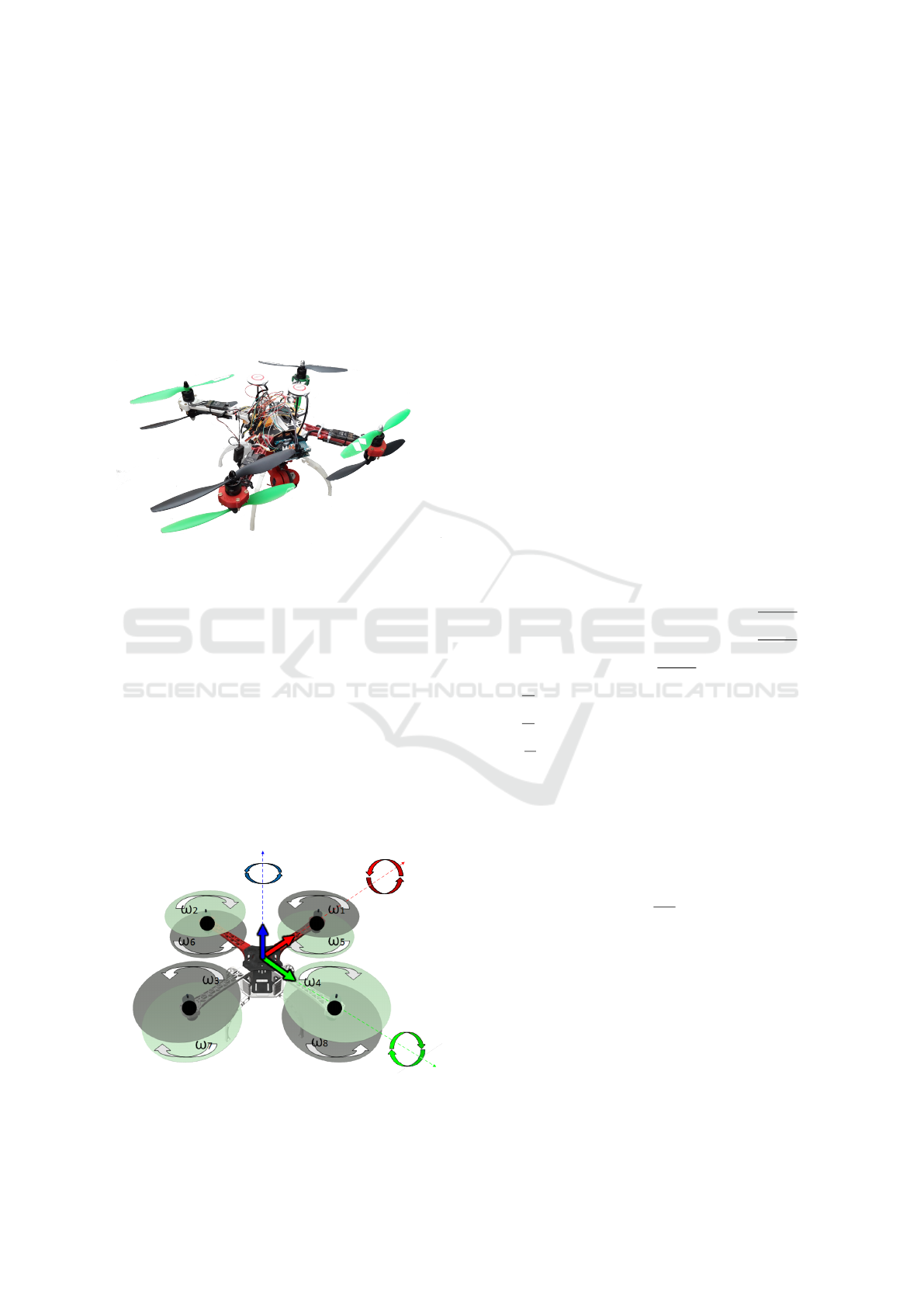
2 MULTICOPTER’S MODEL

The quadcopter’s model, based on the real quadcop-

ter Fig. 1, and the techniques used to model its kine-

matics and dynamics will be brieﬂy explained in this

section.

Figure 1: Quadcopter X8-VB.

Each rotors’ torque and orientation has to be taken

into account to allow the multicopter to hover, move

in three dimensions and rotate in the other three de-

grees of freedom.

∑

n=1

(1)

= f

+ f

− f

(2)

= f

+ f

− f

(3)

= f

+ f

− f

(4)

Figure 2: Representation of the X8 quadcopter. The XYZ

axis and its rotations are represented with RGB colors, re-

spectively.

Equation (1) represents the sum of forces in all ro-

tors, attaining the variation of altitude (Z axis). The

equation (2) refers to the roll (φ) rotation and equa-

tion (3) the pitch (θ) rotation which enable the multi-

copter’s movement in the y and x axis, represented in

Fig. 2 as green and red, respectively. The last equation

(4) refers to the yaw (ψ) responsible for the rotation

around the Z axis, also represented in Fig. 2 as blue.

To obtain the dynamic model of this aircraft, one

must take into consideration its kinematics model, in

other words, its linear and angular position (5), as well

as its linear and angular velocity (6).

Γ =

= [x y z φ θ ψ]

(5)

v =

Ω

= [u v w

ψ]

(6)

These equations represent the twelve states of the

system. Using the Newton-Euler method with the ki-

nematic model to describe the combined translation

and rotational dynamics of the quadcopter, therefore

obtaining its dynamic model represented by the sy-

stem of equations (7).











¨x =



sin(φ)sin(ψ) − cos(φ)cos(ψ)sin(θ)



−F

¨y =



cos(ψ)sin(φ) + cos(φ)sin(ψ)sin(θ)



−F

¨z = −g +



cos(φ)cos(θ)



−F

φ =



− I

)

ψ − J

θω +U



θ =



− I

)

ψ − J

φω +U



ψ =



− I

)

θ +U



(7)

In the set of equations (7), g is the gravity accele-

ration, m is its mass, I

, I

and I

represent the body

inertia in three dimensions, J

is the rotor inertia, ω

is the rotor rotation and, F

, F

and F

(8) are the

drag forces imposed, contrary to its movement.

= C

ρv

A (8)

In equation (8), C refers to the drag coefﬁcient, ρ

the air density, A the impact area with air and v is the

speed.

The system of equations (7) obtained represents

the linear and angular accelerations of the quadcop-

ter and its position and velocity equations can be at-

tained by means of integration (7). For a better un-

derstanding, the ¨x and ¨y accelerations are always de-

pendent on the roll (φ) and pitch (θ) but the yaw (ψ)

makes its appearance if the quadcopter’s referential

in relation to the earth axis is changed rotation wise.

Quadcopter Control Approaches and Performance Analysis

In the ¨z acceleration the yaw (ψ) does not inﬂuence

in any way and the constant acceleration of gravity is

introduced. The last part of ¨x, ¨y and ¨z equations re-

fers to the mass m of the drone, control input U

and

their respective drag forces. The angular accelerati-

ons are inﬂuenced by the drone’s inertial momentum

, I

and J

) as well as its control inputs (U

and U

3 CONTROL APPROACHES

This section will further explain the controllers’ ap-

proaches and algorithms.

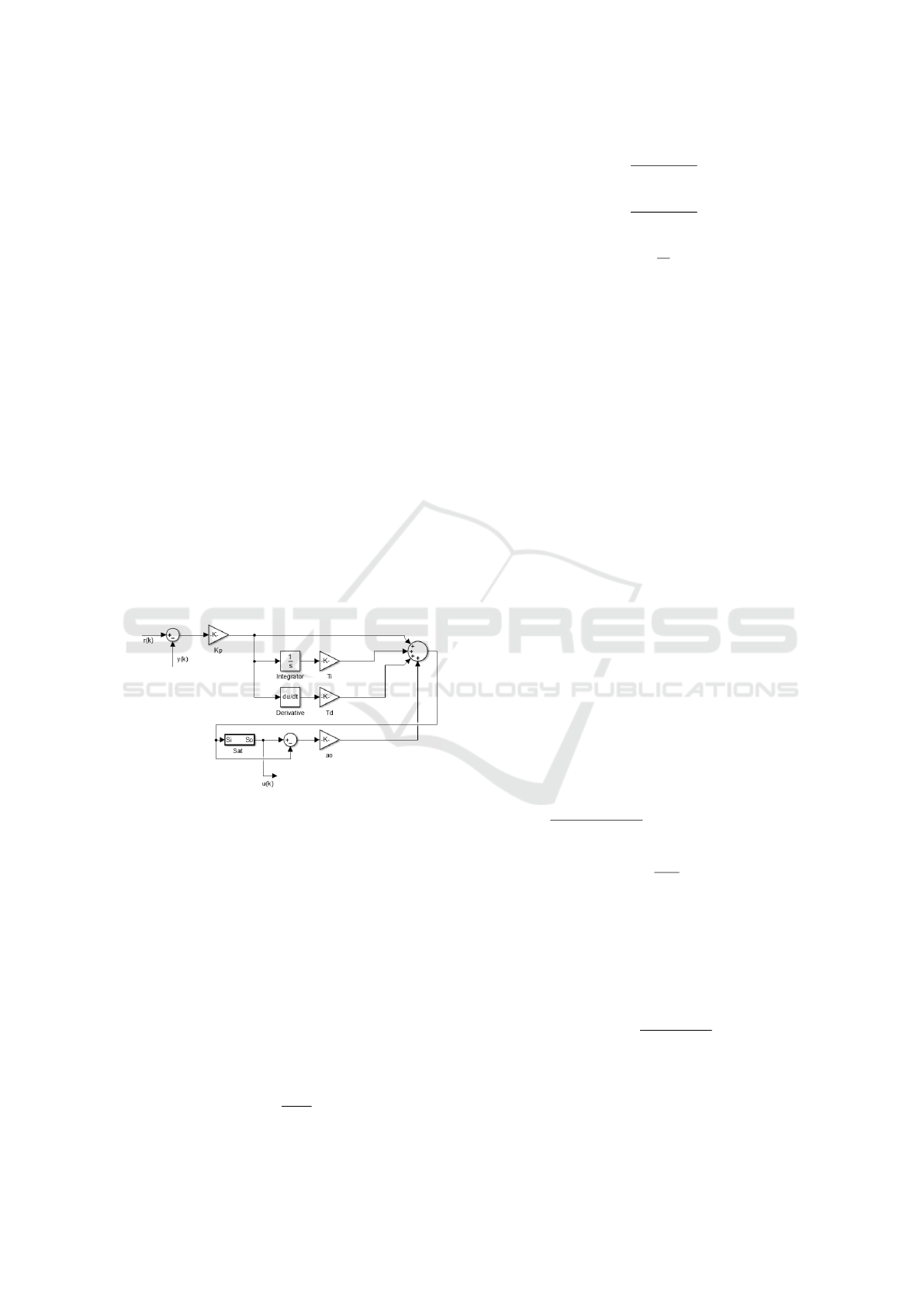
3.1 PID Controller

The Proportional-Integral-derivative controller (PID

Controller) is a very common solution in feedback

control of industrial processes that is meant to force

the process variable to follow the reference taking in

consideration its present (P), past (I) and future (D)

of the error, (Astrom, 1995). The implemented con-

troller’s architecture is represented in Fig. 3, where it

was added an anti-windup term in order to nullify the

integral element’s error accumulation.

Figure 3: PID with anti-windup architecture (continuous-

time).

The implemented PID discrete-time algorithm fol-

lows the equations (9) to (18), where e(k) represents

the control error between the reference r(k) and the

sensor data y(k), bi is the integral gain, ad and bd

are derivative gains, ao is the anti-windup gain, K

is the proportional gain, T

is the sampling time, T

is the integral coefﬁcient, T

is the derivative coef-

ﬁcient, T

is the anti-windup coefﬁcient, P(k), I(k)

and D(k) are the PID controller gains, v(k) is the non-

saturated control actuation and u(k) is the control ac-

tuation with saturation.

e(k) = r(k) − y(k ) (9)

bi =

(10)

ad =

− N T

+ N T

(11)

bd =

N T

+ N T

(12)

ao =

(13)

P(k) = K

e(k) (14)

D(k) = ad D(k − 1)− bd



y(k) − y(k − 1)



(15)

v(k) = P(k) + I(k − 1) + D(k) (16)

u(k) = sat



v(k), ulow, uhigh



(17)

I(k) = I(k − 1) + bi e(k) + ao



u(k) − v(k)



(18)

3.2 Sliding Mode Controller

A Sliding Mode Controller (SMC) is a type of control

that consists in the change of the system state using

a switching function. This technique is very efﬁcient

when dealing with nonlinear systems that can be af-

fected by external disturbances, like aircrafts, (Sh-

tessel et al., 2014), (Spurgeon, 2014), (Utkin et al.,

1999). The controller approach implemented is furt-

her described by the architecture in Fig. 4 and the im-

plemented discrete-time algorithm is deﬁned by the

set of equations (19) to (25), (Palma et al., 2015).

e(k) = r(k) − y(k ) (19)

(k) = g

e(k) − e(k − 1)

+ p

(k − 1) (20)

(21)

(k) = i

(k −1)+T

e(k)+g



u(k −1)−v(k −1)



(22)

(k) = c

(k) + λ i

(k) + d

(k) (23)

v(k) = ρ

(k)

|σ

(k)| + ε

(24)

u(k) = sat



v(k), [0; 1]



(25)

ICINCO 2018 - 15th International Conference on Informatics in Control, Automation and Robotics

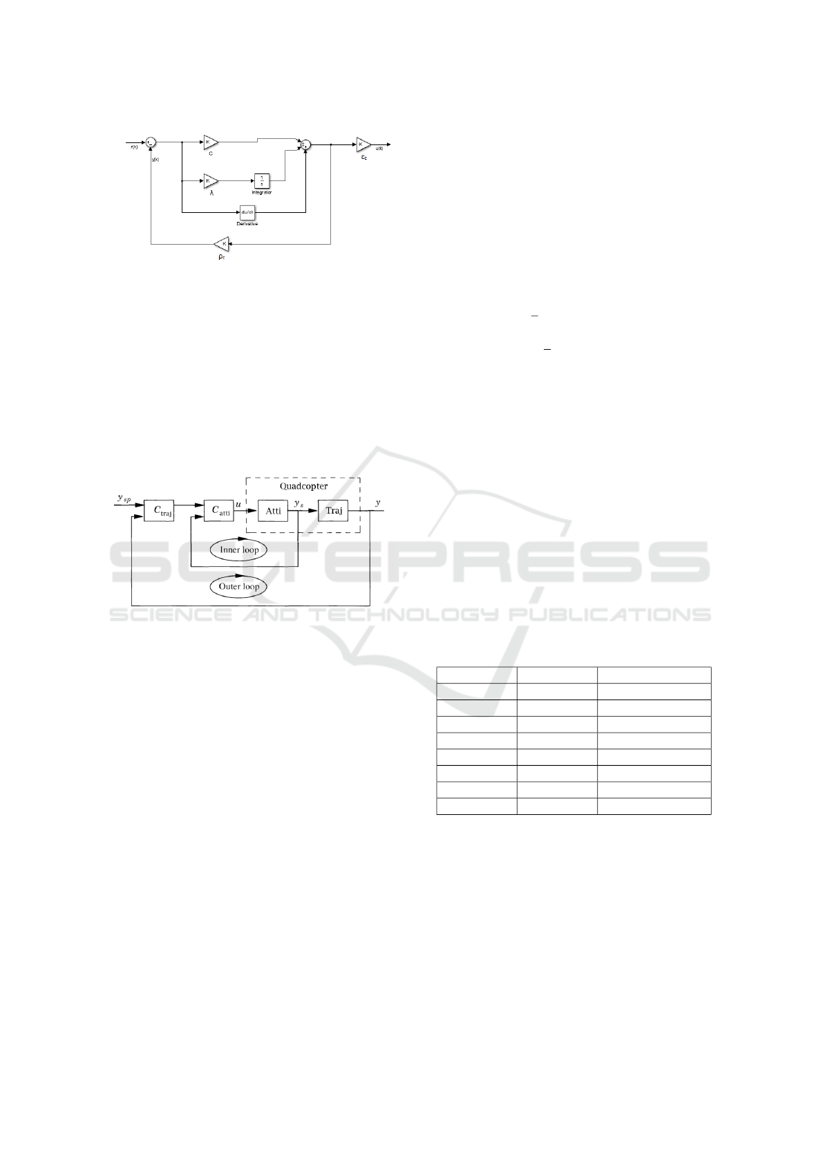
Figure 4: Sliding Mode Controller architecture

(continuous-time).

3.3 Cascade Control

In Fig. 5 the cascade control methodology to move

the quadcopter along the XY plane is illustrated. The

quadcopter will follow the trajectory y

while com-

paring with the current y in the outer loop, by giving

the setpoint to the attitude controller which will fol-

low the desired orientation in the inner loop. The roll

and pitch orientations (inner loop) will affect the mo-

vement in the Y and X axis (outer loop), respectively.

Figure 5: Cascade control for XY plane trajectory.

3.4 Particle Swarm Optimization

The controllers mentioned above were optimized

using the Particle Swarm Optimization (PSO) algo-

rithm, (Palma et al., 2015). This method minimizes

the cost function by optimizing the control parame-

ters, (Kennedy and Eberhart, 1995). The advantage

being that it is not largely affected by the size and

non-linearity of the system, while converging to opti-

mal or sub-optimal solutions where most analythical

methods fail to converge, (Del Valle et al., 2008).

The particles’ respective position p

(k) and speed

(k) on a controller’s parameter space are updated

through equations (26) and (27), (Kennedy and Eber-

hart, 1995), where w, c

and c

are real value parame-

ters, o

(k) and o

are the location of the best position

of the particle i (history) and the best position found

by any particle, respectively. k is the current sample

and rand(.) represents a random value in the range

[0;1].

(k) = p

(k − 1) + s

(k) (26)

(k) = w s

(k − 1)+

rand(.)



(k − 1) − p

(k − 1)



rand(.)



(k − 1) − p

(k − 1)



(27)

In this work, the cost function J

(k) to be minimi-

zed is deﬁned by equation (28), where (k − n + 1 : k)

represents the set of samples of the active control in

a sliding window, mse and var are the control mean-

squared error and the control variance, respectively.

(k) =

mse



e(k − n + 1 : k)



var



u(k − n + 1 : k)



(28)

4 FAULTS AND FAILURES

In this paper, an additive sensor fault was implemen-

ted as well as a failure in motor 1, and thereafter the

controllers behavior was tested in order to evaluate

their robustness.

The actuators failures and its countermeasures

could be determined using equations (1, 2, 3 and 4).

It is important to note that the system is able to to-

lerate these failures because of the X8 architecture’s

fault/failure tolerant proprieties.

Taking into account the studies in (Brito et al.,

2016) one can obtain the Table 1 regarding the actua-

tors faults and the action to take in each case, (Brito,

2016).

Table 1: Motor failure and reconﬁguration.

Failure Recon f . Control Retuning

Motor 1 Motor 7 Pitch, Yaw

Motor 2 Motor 8 Roll, Yaw

Motor 3 Motor 5 Pitch, Yaw

Motor 4 Motor 6 Roll, Yaw

Motors 1, 3 Motors 2, 4 Pitch, Roll, Yaw

Motors 2, 4 Motors 1, 3 Pitch, Roll, Yaw

Motors 5, 7 Motors 6, 8 Pitch, Roll, Yaw

Motors 6, 8 Motors 5, 7 Pitch, Roll, Yaw

In Table (1), the reconﬁguration column shows the

rotor(s) to disable in case of the failure in the ﬁrst co-

lumn rotor. The third column regards the controllers

that need to be adjusted according to each new actua-

tors conﬁguration.

5 SIMULATION RESULTS

The simulation results showing the controllers’ beha-

vior will be presented in this section, and so will be

Quadcopter Control Approaches and Performance Analysis

their respective gains. The sampling period used in

the simulations was 0.1 s. Part of the position and

orientation variables are normalized between [-1, 1]

and others are between [0, 1].

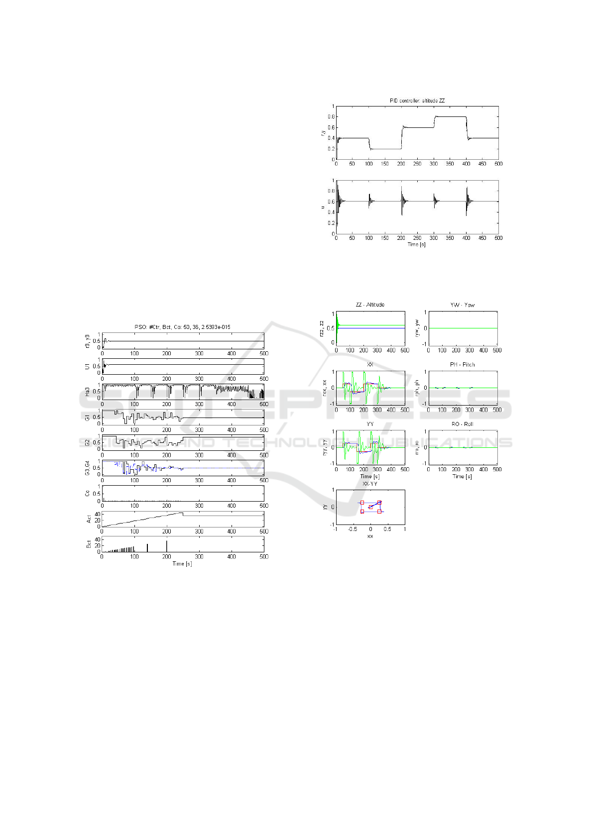
5.1 Controller’s Optimization based on

PSO

Fig. 6 illustrates the PSO algorithm’s iterations to op-

timize the gains of a controller. From top to bottom

can be observed the altitude(y3) and its reference(r3),

U1 is the control action, Ha3 is the Harris index

(Brito Palma et al., 2013), G1, G2, G3 and G4 are the

gains associated with the controller, Co is the value

of the cost function, Act is the active controller and

Bct is the best controller found at the moment. Fig. 6

presents the PSO algorithm for the sliding mode con-

troller, in which, from 50 controllers the 36th was the

best, presenting a cost function value of 2.5393e+15.

Figure 6: PSO algorithm for the sliding mode controller.

5.2 PID Controller

The PID gains obtained from the PSO optimiza-

tion process around a setpoint of 0.5 were: K

2.7272, T

= 4.224 and T

= 1.0356.

In Fig. 8 can be observed the movement of the

quadcopter along a square trajectory for a constant

altitude of 0.5. The movement in the XY plane has

a direct correlation with the pitch and roll orientation

of the drone. This means that leaning the quadcopter

forward and backward (pitch) enables the movement

Figure 7: PID simulation result.

in the X axis. Likewise, leaning sideways enables the

movement in the Y axis.

Figure 8: PID simulation results for trajectory and orien-

tation tracking (red is the setpoint, blue is the output and

green is the control action.

In Fig. 7 the set of references was [0.4, 0.2, 0.6,

0.8, 0.4], where r (reference) and y (sensor data) are

represented in the graphic above and the u (control ac-

tuation) below, which represents a nominal hovering

situation.

5.3 Sliding Mode Controller

The gains obtained for the SMC controller after op-

timization around the setpoint of 0.5 were: c =

7.1163, λ = 7.7377, g

= 16.4048, ρ = 5.3944, ε

18.7194 and p

= 0.2553.

ICINCO 2018 - 15th International Conference on Informatics in Control, Automation and Robotics

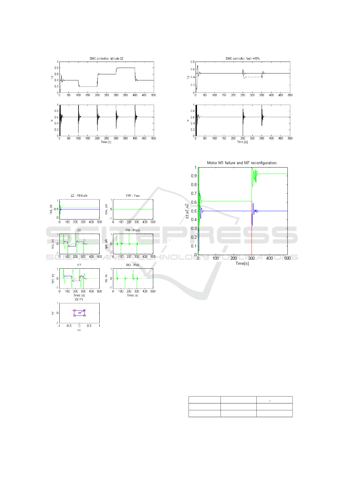
Figure 9: Sliding Mode Controller simulation result.

In Fig. 10 the same trajectory in the XY plane was

simulated. The sliding mode controller presents a fas-

ter dynamic than the PID due to its nonlinear beha-

vior, as depicted in pitch and roll ﬁgures.

Figure 10: Sliding Mode Controller simulation results for

trajectory and orientation tracking.

In the Fig. 9 the r (reference) and y (sensor data)

are represented in the graphic above and the u (control

actuation) below. The same reference [0.4, 0.2, 0.6,

0.8, 0.4] was deﬁned for this simulation and it also

demonstrates a nominal hovering situation.

The Fig. 11 shows the behavior of the SMC when

in the presence of a 10% additive abrupt fault above

and its respective control actuation below.

In Fig. 12 a fault in motor 1 can be observed as

well as its reconﬁguration by disabling the motor 7 at

Figure 11: Sliding Mode Controller with fault simulation.

Figure 12: Fault in motor 1 and reconﬁguration by disabling

motor 7.

300 seconds when the drone loses altitude. After the

reconﬁguration the thrust lost from the disabled mo-

tors has to be compensated by the other motors (their

control action increases from 0.6 to 0.9).

5.4 Controllers Performance

Comparison

Table 2 presents the performance indexes mean-

squared error (MSE) and variance of control action

(Var

) in altitude (Fig. 7 and Fig. 9).

Table 3 presents the performance indexes mean-

squared error (MSE) and the variance of control

Table 2: Controller performance comparison with SP = [0.4

0.2 0.6 0.8 0.4] in altitude.

Controller MSE Var u

PID 1.0903e-003 2.7262e-003

SMC 2.2237e-003 5.9492e-003

Quadcopter Control Approaches and Performance Analysis

Table 3: Controller performance for sensor fault recovery in

altitude.

Controller MSE Var u

PID 1.5060e-003 2.8384e-003

SMC 3.3218e-003 3.9561e-003

action (Var

), for an additive faulty sensor situation

(+10%).

From the graphics one must observe that both con-

trollers serve their intent maintaining the altitude and

responding to the different amplitude steps.

It is important to note that the non-linear SMC

controller has more control variance than the linear

PID controller because it has a faster response time

and has some chattering. The linear PID controller

demonstrates a slight better overall performance since

it is working around a linear operating point.

Although the controllers performance indexes ob-

served in Table 2 and 3 are similar, one can conclude

that, in case of an additive sensor fault, the PID con-

troller shows a better response in relation to the no-

minal behavior than the SMC. It is also noticeable

that, the control variance (Var u) of the SMC is not

affected by the sensor fault, it even decreases its va-

lue.

Table 4: Controller performance comparison with square

setpoint in the XY plane.

Controller MSE(X) + MSE(Y )

PID 0.0297

SMC 0.0217

Without faults, the XY trajectories related with the

PID and SM controllers were compared using a per-

formance index given by the sum of the mean square

error (MSE) according to the X axis plus the MSE

according to the Y axis.

The trajectory tracking of the PID and Sliding

Mode controllers present some overshoot, due to their

pure feedback architectures, which is not desired for

quadcopter path following. Differential Flatness con-

trol allows a null overshoot and near perfect tracking

of the desired orientations and trajectories, thanks to

its feedforward aspect that preemptively calculates

the best actuations for each trajectory (Brito et al.,

2018).

6 CONCLUSIONS

In this paper, fault tolerant control approaches of a

quadcopter model with X8 conﬁguration were presen-

ted.

The particle swarm optimization (PSO) algorithm

reveals a good approach to obtain sub-optimal con-

trollers, as an optimal one would require a lot of com-

putational time and effort.

According to the simulation results, both control-

lers (PID and SMC) were able to fulﬁll their control

and tracking tasks.

Regarding the altitude trajectory tracking, both

controllers presented similar performance.

The Sliding Mode Controller presents a better per-

formance in the XY trajectory tracking.

The fault tolerant architecture presented an

efﬁcient reconﬁguration of the system when in

faulty situations, in which the quadcopter conti-

nues to ﬂy when faults/failures happened in the sen-

sors/actuators.

Future work will take into account the overshoot

in the performance index of the PSO optimization in

order to improve the trajectory tracking.

ACKNOWLEDGEMENTS

This work has been supported by Departamento de

Engenharia Eletrotecnica of Faculdade de Ci

encias

e Tecnologia of Universidade Nova de Lisboa, by

Uninova-CTS research unit, by CISUC research unit

and by national funds through FCT - Fundac

ao para

a Ci

encia e a Tecnologia within the research unit

CTS - Centro de Tecnologia e Sistemas (project

UID/EEA/00066/2013). The authors would like to

thank all the institutions.

REFERENCES

Astrom, K. J. (1995). PID controllers: theory, design and

tuning.

Blanke, M., Kinnaert, M., Lunze, J., and Staroswiecki, M.

(2006). Diagnosis and Fault-Tolerant Control.

Bouabdallah, S. and Siegwart, R. (2005). Backstepping and

Sliding-mode Techniques Applied to an Indoor Micro

Quadrotor. In Proceedings of the 2005 IEEE Interna-

tional Conference on Robotics and Automation, pages

2247–2252. IEEE.

Brito, A., Brito, V., Palma, L. B., Coito, F., and Gil, P.

(2018). Trajectory control approaches for a fault to-

lerant quadcopter. In 2018 International Young Engi-

neers Forum (YEF-ECE), pages 13–18. IEEE.

Brito, V. (2016). Fault Tolerant Control of a X8-VB Quad-

copter. Msc, FCT-UNL.

Brito, V., Brito Palma, L. F. F., Vieira Coito, F., and Val-

tchev, S. (2016). Modeling and Supervisory Control

of a Virtual X8-VB Quadcopter. In 17th International

Conference on Power Electronics and Motion Control,

page 8, Varna, Bulg

aria.

ICINCO 2018 - 15th International Conference on Informatics in Control, Automation and Robotics

Brito Palma, L., Moreira, J., Gil, P., and Coito, F. (2013).

Hybrid Approach for Control Loop Performance As-

sessment. KES-IDT - 5th International Conference on

Intelligent Decision Technologies, 2013.

Del Valle, Y., Venayagamoorthy, G. K., Mohagheghi, S.,

Hernandez, J.-C., and Harley, R. G. (2008). Particle

Swarm Optimization: Basic Concepts, Variants and

Applications in Power Systems. Evolutionary Com-

putation, IEEE Transactions on, 12(2):171–195.

Isermann, R. and Ball

e, P. (1997). Trends in the applica-

tion of model-based fault detection and diagnosis of

technical processes. Control Engineering Practice,

5(5):709–719.

Kennedy, J. and Eberhart, R. (1995). Particle swarm opti-

mization. Neural Networks, 1995. Proceedings., IEEE

International Conference on, 4:1942—-1948 vol.4.

Leong, B. T. M., Low, S. M., and Ooi, M. P. L. (2012).

Low-cost microcontroller-based hover control design

of a quadcopter. In Procedia Engineering, volume 41,

pages 458–464.

Luukkonen, T. (2011). Modelling and Control of Quadcop-

ter. Journal of the American Society for Mass Spectro-

metry, 22(7):1134–1145.

Merz, T. and Kendoul, F. (2013). Dependable low-altitude

obstacle avoidance for robotic helicopters operating in

rural areas. Journal of Field Robotics, 30(3):439–471.

Mustapa, Z., Saat, S., Husin, S. H., and Abas, N. (2014). Al-

titude controller design for multi-copter UAV. In 2014

International Conference on Computer, Communicati-

ons, and Control Technology (I4CT), pages 382–387.

IEEE.

Palma, L. B., Coito, F. V., Ferreira, B. G., and Gil, P. S.

(2015). PSO based on-line optimization for DC mo-

tor speed control. In 9th International Conference on

Compatibility and Power Electronics, CPE 2015, pa-

ges 301–306.

Shtessel, Y., Edwards, C., Fridman, L., and Levant, A.

(2014). Sliding Mode Control and Observation. Con-

trol Engineering. Springer New York, New York, NY.

Spurgeon, S. (2014). Sliding mode control : a tutorial. Proc.

of the European Control Conference (ECC), 2014,

(1):2272–2277.

TIME (2015). How Drones Are Already Being Used to

Help Save People.

Utkin, V., Guldner, J., and Shi, J. (1999). Sliding mode

control in electro-mechanical systems.

Yih, C.-C. (2016). Flight control of a tilt-rotor quadcop-

ter via sliding mode. In 2016 International Automatic

Control Conference (CACS), pages 65–70. IEEE.

Quadcopter Control Approaches and Performance Analysis