Coevolutionary Algorithm for Multivariable Discrete Linear

Time-variant System Identiﬁcation

Alexander E. Robles and Mateus Giesbrecht

School of Electrical and Computer Engineering, University of Campinas, Av. Albert Einstein 400, Campinas - SP, Brazil

Keywords:

Evolutionary Algorithms, Coevolutionary Algorithms, System Identiﬁcation, Time-variant System Identiﬁca-

tion.

Abstract:

A signiﬁcant part of the works in system identiﬁcation is focused on time-invariant dynamic systems. How-

ever, most of systems in the real applications have nonlinear and time variant behavior. In this paper, we

present a multivariable time-variant identiﬁcation method based on a paradigm in the ﬁeld of evolutionary

algorithms: The coevolutionary algorithm. This new method focuses on the relationship between the ﬁtness of

an individual in relation to the ﬁtness of the other individuals (or group of individuals), based on the principle

of the selective pressure, that is part of the evolutionary process. A brief comparison between a multivariable

deterministic identiﬁcation method MOESP-VAR and the proposed coevolutionary method is shown. From

the results it is possible to notice that the proposed method presents an accuracy higher than the obtained with

the deterministic identiﬁcation method.

1 INTRODUCTION

System identiﬁcation consists on ﬁnding the math-

ematical models that can describe dynamic systems

behavior, from observed input-output data (Ljung,

1999). A signiﬁcant part of activities and researches

in system identiﬁcation focuses on time-invariant dy-

namic systems. However, there are innumerable sys-

tems in nature that are multivariable with nonlinear

and time-varying behavior. To deal with last problem,

many of the time-varying systems are approximated

by linear time-invariant systems, as long as these sys-

tems vary slowly (Tamariz et al., 2005). In some cases

these approximations cannot describe the real variant

system behavior, so that the magnitude of the error be-

tween output data and output model is considerable.

The main focus of this paper is to present an

evolutionary method to identify multivariable time-

varying system (MTVS). For decades evolutionary

algorithms (EAs) have been applied in optimization

problems with successful results. Moreover, system

identiﬁcation area had one of its ﬁrst applications in

(Rodrigues-Vasquez and Fleming, 2004) when a clas-

sical genetic algorithm is applied to identify the pa-

rameters of the transfer function of a two masses res-

onant system. In (Wakizono and Uosaki, 2006) an ap-

proach for identifying linear and non-linear systems

based on CLONALG algorithm (De Castro and Von

Zuben, 2002) was proposed. Other recent work is

(Giesbrecht and Bottura, 2015), in which an immuno-

inspired algorithm was develop to identify MTVS. In

that reference, the MTVS identiﬁcation problem is

deﬁned as an optimization problem, where a search

space is created by all possible matrices quadru-

ples A,B,C, D that represent the MTVS in state-space

model for a given time interval. Furthermore, each

state-space model is seen as a point that minimizes the

error between the system and the model outputs to the

same input signal. In this paper, those principles were

used to develop the coevolutionary algorithm (COEA)

that can be applied to MTVS identiﬁcation problem.

In this work, some comparisons are made between

implemented COEA and deterministic method called

MOESP-VAR (Tamariz et al., 2005), based on Multi-

variable Output-Error State sPace (MOESP) (Verhae-

gen and Dewilde, 1992). A genetic algorithm (GA)

also was implement using the same parameters and

operators used for COEA, but the populations do not

evolve together. Trying to show the effectiveness of

evolutionary processes, it was developed a random

search (RS), that performs a searching without any

evolutionary intelligence behind.

The paper is organized as follows. In the next sec-

tion, subspace methods for system identiﬁcation are

introduced. In the section 3, the coevolutionary algo-

rithms are brieﬂy detailed. Section 4 describes COEA

to identify MTVS, where the coevolution is the main

topic. In the section 5 the results of the application

290

Robles, A. and Giesbrecht, M.

Coevolutionary Algorithm for Multivariable Discrete Linear Time-variant System Identiﬁcation.

DOI: 10.5220/0006907602900295

In Proceedings of the 15th International Conference on Informatics in Control, Automation and Robotics (ICINCO 2018) - Volume 1, pages 290-295

ISBN: 978-989-758-321-6

of the proposed method to identify a discrete slowly

time-varying benchmark are shown. In the same sec-

tion we compare COEA with other approaches such

as GA, RS, and MOESP-VAR method. Finally, in

the section 6, the conclusions of this paper and future

works are exposed.

2 SUBSPACE METHODS FOR

SYSTEM IDENTIFICATION

2.1 State-space Models

A multivariable system can be modeled in state-

space representation. The discrete multivariable time-

invariant system is deﬁned in state-space model as fol-

lows:







x(k + 1) = Ax(k) + Bu(k)

y(k) = Cx(k) + Du(k)

(1)

Where x(k) ∈ R

is deﬁned as the system state at

instant k, A ∈ R

nXn

is the state transition or system

matrix, B ∈ R

nXm

is a matrix that relates the input

u(k) ∈ R

to the state, C ∈ R

lXn

is the matrix that

relates the output y(k) ∈ R

to the state and D ∈ R

lXm

is the matrix that relates the outputs to the inputs

(Katayama, 2005), (Ljung, 1999).

2.2 Subspace Methods for System

Identiﬁcation

Multivariable discrete system identiﬁcation using

subspace methods allows ﬁnding a causal time-

invariant model (1). The model is estimated just from

system outputs and inputs. The main advantage of

this approach is that a MIMO system can be mod-

eled even if the system order is unknown a priori.

There are well known subspace methods to address

the time-invariant MIMO system identiﬁcation such

as MOESP and N4SID. The MOESP method (Ver-

haegen and Dewilde, 1992) is based on the LQ de-

composition of Hankel matrix formed from input-

output data, where L is lower triangular and Q is or-

thogonal. A Singular Value Decomposition (SVD)

can be performed on a block from the L matrix to

obtain the system order and the extended observabil-

ity matrix. From this matrix it is possible to estimate

the matrices C and A of model (1). The ﬁnal step

is to solve overdetermined linear equations using the

least-squares method to estimate matrices B and D,

for more details see (Giesbrecht and Bottura, 2015).

Another method is N4SID (Numerical Algo-

rithms for Subspace State Space System Identiﬁca-

tion) (Overschee and Moor., 1994). The method stars

with the oblique projection of the future outputs to

past inputs and outputs into the future inputs direc-

tion. The second step is to apply the LQ decomposi-

tion and then the state vector can be computed by the

SVD. Finally, it is possible to compute the matrices

A,B,C and D by using the least-squares method.

2.3 Time-varying Systems

Most of the systems in real environments are nonlin-

ear and time-variant, so the complexity of the system

identiﬁcation problem increases. Time-varying sys-

tems can be modeled in state-space as shown in (2),

where the matrices A, B,C, D depend on k, that repre-

sents the time.







x(k + 1) = A(k)x(k) + B(k)u(k)

y(k) = C(k)x(k) + D(k)u(k)

(2)

There is a MOESP type method called MOESP-

VAR. This method was develop in (Tamariz et al.,

2005). Given a slowly time-varying system, the al-

gorithm starts splitting up the output-input data into

intervals deﬁned as windows. Then, the MOESP al-

gorithm is applied to each window and the matrices

A,B,C,D are estimated. If the system presents a fast

variation, the MOESP-VAR algorithm has poor ac-

curacy. Another disadvantage is that the matrix de-

compositions used in the subspace methods is limited

by the size of window data, in other words a greater

amount of data is needed in order to make new meth-

ods are computationally feasible. For this case, tech-

niques based on EAs can be used as an alternative, as

proposed in (Giesbrecht and Bottura, 2015).

3 SYSTEM IDENTIFICATION

PROBLEM AS A

OPTIMIZATION PROBLEM

The identiﬁcation of time variant systems can be de-

ﬁned as an optimization problem if a space of state

space models is deﬁned. The space contains all possi-

ble quadruples of matrices, the dimensions of matri-

ces being known a priori. Each model in the state

space is seen as a point in this space, also called

search space. The main idea is to ﬁnd the point that

minimizes the error between the model and system

outputs generated from the same input. This point

also changes over time, that is, another quadrupling

of matrices must be estimated.

EAs can adapt well to this optimization problem.

For larger system variations over time, the algorithm

Coevolutionary Algorithm for Multivariable Discrete Linear Time-variant System Identiﬁcation

291

should look for a new, four-point point that minimizes

the estimation error. Based on this principle the CO-

EAs were developed in this paper. In an illustrative

way, the optimization problem can be deﬁned as fol-

lows:

Exists X

∈ R

(n+p)X (n+m)





(3)

The estimation error E(X

) is calculated in equa-

tion 4 and the ﬁtness function f (X

) is deﬁned in

equation 5. Where y(k) is the system output, ˆy(k)

is the model output (estimated by evolutionary algo-

rithm) and N is the data size.

E(X

) =

∑

k=1

||(y(k) − ˆy(k))|| (4)

f (X

) =

1 + E(X

)

(5)

There is a x

∗

which minimizes error, this concept

taken to the ﬁtness function, means to maximize the

ﬁtness function and is deﬁned: x

∗

→ max( f (x

∗

)). The

equation 5, can be modiﬁed or changed, this is an-

other advantage of the EAs, which does not restrict

the ways of creating a new ﬁtness function.

4 COEVOLUTIONARY

ALGORITHMS

Coevolutionary algorithms (COEAs) are heuristic

methods based on cooperation and competition.

Moreover, coevolution is strongly associated with a

mutual evolution between two species, so that one ex-

erts selective evolutionary pressure on the other, thus

creating a paradigm: there is no isolated evolution.

More detailed information regarding this subject can

be found in the reference (Wiegand, 2003).

There are three categories that might beneﬁt from

coevolution: problems with large (inﬁnite) Cartesian-

product spaces, problems with no intrinsic objective

measure, and problems with complex structures. The

intent of coevolution is to produce a typical dynamic

refereed as an arms race. The idea is that continued

small adaptations in some individuals (or populations)

will force competitive adaptations in others. Con-

sider the predator-prey systems: if the prey evolves

to run faster; then the predator population is forced

to develop better attacking strategies (such as power-

ful claws). Therefore, the expectation is that, as the

processes evolves, both populations will present ex-

ceptional attributes (Wiegand, 2003).

Another concept, used in this work, is the cooper-

ative. In a context in which a large problem is very

complex to solve, it may be possible to divide the

problem into subcomponents and to solve each one

of them independently. The subcomponents are also

deﬁned as subpopulations and the only interaction be-

tween subpopulations is in the cooperative evaluation

of each individual of this subpopulations. This is done

by concatenating the current individual with the best

individuals from the rest of the other subpopulations,

as described by (Potter and Jong, 2000).

Indeed, the advantages of the coevolution led this

kind of technique to be applied in a large variety

of complex problems. Optimization applications in-

clude the coevolution of fast, complete sorting net-

works (Hillis, 1991) and the coevolution of maximal

arguments for complex functions (Potter and Jong,

1994). Machine learning applications include COEAs

to search for useful game-playing strategies (Rosin

and Belew, 1996).

5 COEVOLUTIONARY

ALGORITHM TO SYSTEM

IDENTIFICATION

Based on the principles of cooperative coevolution, in

this work a COEA was develop to identify MTVS. To

initialize the algorithm four populations were created:

, P

and P

, that are related to the matrices A, B,

C and D from the state-space model (2), respectively.

Notice that these matrices are not constant.

The individual objective of the populations is to

ﬁnd the conﬁguration of their associated state matri-

ces, that minimizes the estimation error between the

model outputs

Y and the actual system outputs Y to

the same given input set U . The search space for each

state-space matrix (2) is M

∈ R

nXn

∈ R

nXm

∈

lXn

, M

∈ R

lXm

. The populations belong to those

search spaces.

In the following subsections the adopted coding,

operators, the ﬁtness function and the structure of al-

gorithm are introduced.

5.1 Adopted Coding

The candidate solutions of each population is rep-

resented as follows: P

has nXn elements, P

has

nXm elements, P

has lX n elements P

has lX m el-

ements. The columns of each state-space matrix are

transformed to rows and concatenated. This coding is

shown for P

in the table 1. The other matrices follow

the same coding.

ICINCO 2018 - 15th International Conference on Informatics in Control, Automation and Robotics

292

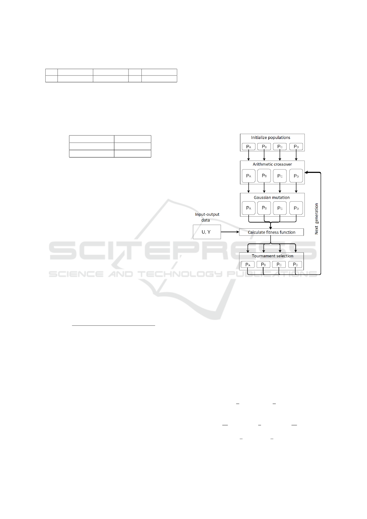
Table 1: Conﬁguration of P

chromosome.

1→n,1

1→n,2

··· a

1→n,n

1,1

→ a

n,1

) (a

1,2

→ a

n,2

) ··· (a

1,n

→ a

n,n

)

5.2 Operators

The four populations P

, P

and P

used the same

operators, which are shown in the table 2.

Table 2: Operators.

Recombination Arithmetic

Mutation Gaussian

Selection Tournament

In the mutation, the value of the variance depends

on the number of generations, see 3. This approach

was inspired by the simulated annealing (Kirkpatrick

et al., 1983), where it is desired that individuals have

greater freedom to explore the search space during

the ﬁrst generations. As the generations (g) pass, the

freedom of exploration should be reduced, to encour-

age individuals to reﬁne the candidate solutions pre-

viously encountered. In the original simulated an-

nealing, the decay of this exploration factor (called

temperature T ) acts on the selection of individuals,

whereas in this work it acts on the mutation of in-

dividuals, generating a reduction in the intensity of

mutations over time.

The reduced value of individuals for tournament

selection, generates low selective pressure in the pop-

ulation, as a consequence, allows low ﬁtness individ-

uals have a high chance to survive.

5.3 Fitness Function

The ﬁtness function is deﬁned as follows:

f (p

(A,i)

) =

1 + E(p

(A,i)

, p

(B,r

), p

(C,r

)

, p

(D,r

)

(6)

Where individual p

(x,i)

of population x, in last

equation (6) corresponds to P

. Also, r

, r

and r

are random individuals extracted from the others pop-

ulations. The function E represents the total error be-

tween the model outputs ˆy(k) estimated from these

individuals and the system outputs y(k), where n is

the total number of data samples set to be considered.

This function is deﬁned as follows:

E(p

(A,i)

, p

(B,r

)

, p

(C,r

)

, p

(D,r

)

) =

∑

k=1

||(y(k) − ˆy(k)||

(7)

5.4 Structure

The ﬁrst step is to initialize randomly the individuals

from each population. The number of candidate solu-

tions that are selected for mutation and recombination

has deterministic behavior, in which 75% of the pop-

ulation is selected for the crossover, while 25% of the

individuals undergo mutation. Then, the ﬁtness of the

individuals is calculated. Finally, the step of selection

is made. All steps are shown in Figure 1.

Figure 1: Algorithms steps.

6 RESULTS

In the following example the algorithm proposed in

this paper was applied to identify a slowly time-

varying system. A bi-dimensional white noise with

N = 1000 samples was given as input. The parame-

ters of the algorithm were conﬁgured as shown in the

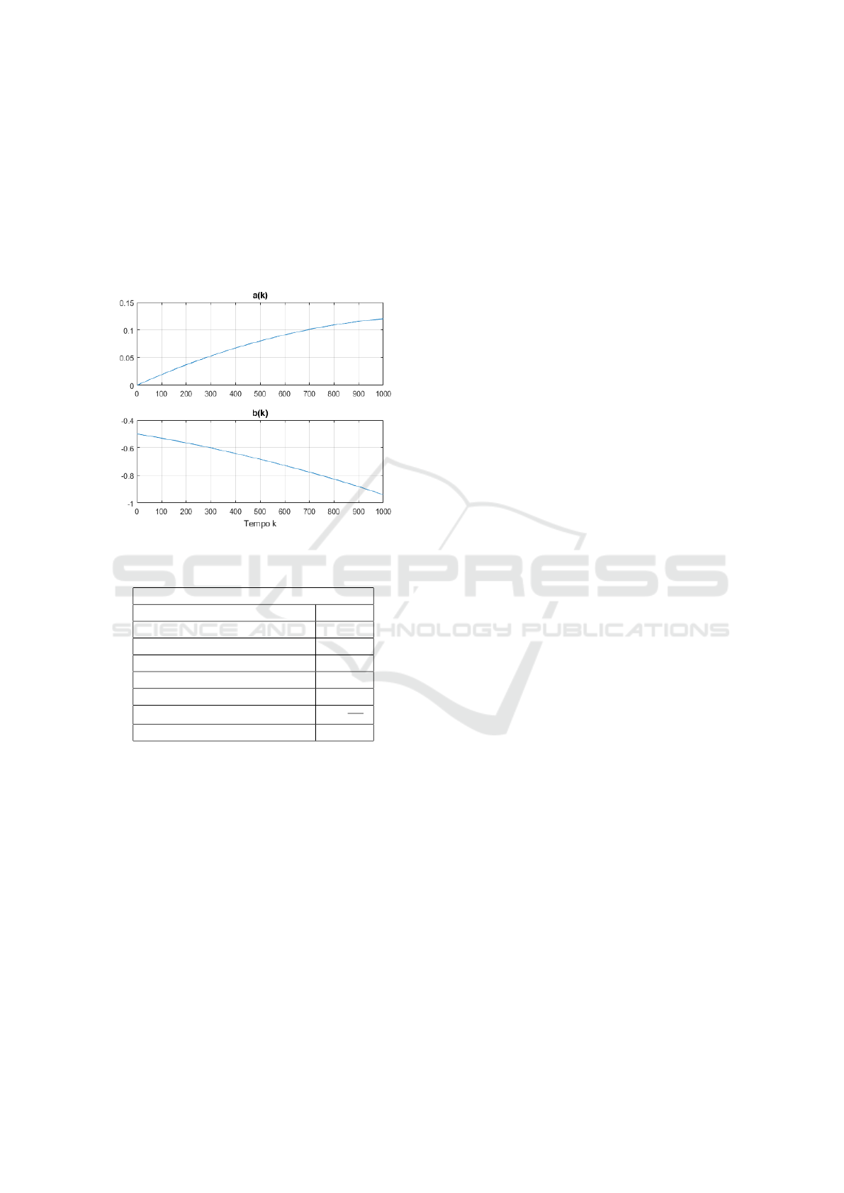
Table 3. The benchmark is modeled by the following

model taken from (Tamariz et al., 2005):



a(k) b(k)

1 −1



(8)

where

a(k) = −

(k/2500)

b(k) = −

(k/2500)

−

(k/2500)

−

(k/2500)

−

(k/2500) −

Coevolutionary Algorithm for Multivariable Discrete Linear Time-variant System Identiﬁcation

293

The others matrix are invariant



−2 1

1 1



; C



1 3

1 2





1 3

1 1



(9)

The time variation of the parameters a(k) and b(k)

are shown in Figure 2.

Figure 2: Time variations in the parameters of A

Table 3: Parameters conﬁguration.

Parameters

Number of populations 4

Generations (g) 4000

Size of population 200

Individuals to crossover 150

Selection probability (α) 0.6

Individuals to mutation 50

Variance (σ) 1 −

2∗g

Individuals to tournament (q) 2

In the process of identifying systems using coevo-

lution, diversity is a key factor to ensure the evolu-

tion progress. Often the increase in ﬁtness is not as-

sociated to the best ﬁtness individual. For instance,

the chromosome with the highest ﬁtness population

will not necessarily get better ﬁtness when in-

teracting with the best individual of the population

. Increased ﬁtness can happen through interactions

between a high ﬁtness individual and another from

below or even between two low ﬁtness individuals.

Thus, ensuring the population diversity through regu-

lar mutations is crucial to its evolution.

Interdependence among populations is a limiting

factor affecting the evolutionary progress of a pop-

ulation. For example, if a population has already

found the optimal solution within their search space,

it will not help if the other populations do not evolve

together. For this reason, the progress of a popula-

tion usually triggers the progress of other populations.

This can be seen in Figure 3, in which the ﬁtness evo-

lution of the four populations along the iterations is

presented. From the ﬁgure it is possible to perceive

that the interdependence of the populations occurs

during the generations of 2000 to 3400, where the ad-

vance of a population, that affects the others happens.

The number of generations was determined by empir-

ical analysis. It has been realized that the populations

need at least 4000 generations to obtain relevant ﬁt-

ness values.

To evaluate the proposed method, the data gener-

ated by white noise (N = 1000) was divided into 5

sets: (U

),(U

) and (U

In those sets, the system variation is higher for the

higher index data. For instance, the variation for

) is greater than those of (U

) and less than

). In each data set, three additional methods

were applied: MOESP-VAR, GA and RS. To ensure a

fair evaluation, the number of iterations (generations)

made for each method, except for MOESP-VAR, was

the same. In addition, GA uses the same operators

and parameters applied to COEA.

The results are presented in the Table 4. It is possi-

ble to infer that MOESP-VAR and COEA have simi-

lar performance, but in most cases the coevolution has

a slight advantage. This may be a promising result

which indicates that more elaborate reﬁnement may

lead to coevolution to ﬁnd the solution even better for

time-varying system identiﬁcation problem.

Both GA and RS have ﬁtness ten times lower than

MOESP-VAR and COEA, this occurs because GA

and RS try to ﬁnd the best conﬁguration of the sub-

spaces at once, that is, they work with the evolution of

individuals with dimension 16. On the other hand, co-

evolution uses the idea of ”divide for conquer ”, where

different populations try to ﬁnd the sub-solutions that

interact better with the other individuals of other pop-

ulations.

7 CONCLUSIONS

In this paper the steps to identify time-varying sys-

tems with COEA are deﬁned. The results have

demonstrated that this type of algorithm has bet-

ter performance (ﬁtness) than deterministic method

MOESP-VAR in the majority of the examples stud-

ied. Moreover, this approach estimates models of

time-varying systems, which represent the system in a

window or time interval. In addition, the coevolution

allows to parallelize the evolutionary process, which

can make it competitive in terms of execution time.

ICINCO 2018 - 15th International Conference on Informatics in Control, Automation and Robotics

294

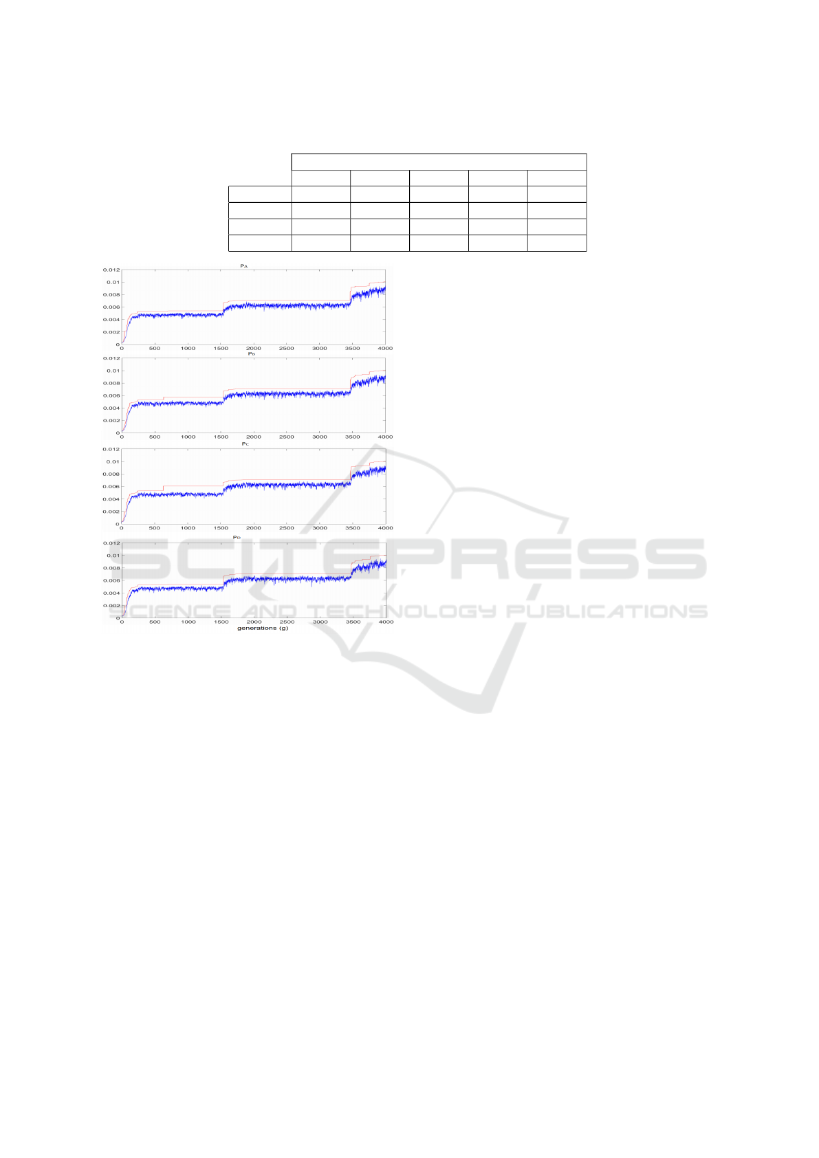
Table 4: Fitness value of the best individual for the data sets used in each method.

Fitness (x10

−3

)

) (U

)

COEA 10.1 6.2 5.4 5.1 2.2

MOESP-VAR 8.23 6.51 5.33 4.27 2.13

GA 0.97 0.78 0.85 0.83 0.67

RS 0.82 0.65 0.81 0.61 0.52

Figure 3: Fitness of the four populations for (U

) set .

The red curve represents the ﬁtness of the best individual

(best ﬁtness) and the blue curve is the mean ﬁtness of the

population.

The main objective was to ﬁnd the matrices

D (state-space model), that minimize the es-

timation error by solving an optimization problem. A

new approach for future work would be to develop a

recursive coevolution method, to estimate the state-

space model at each instant of time. Other evolution-

ary techniques can be implemented to ﬁnd the best

alternative to solve the deﬁned optimization prob-

lems. Finally, the proposed method can be applied to

model time series and compare results with immuno-

inspired algorithm (Giesbrecht and Bottura, 2015).

REFERENCES

De Castro, L. N. and Von Zuben, F. J. (2002). Learning and

optimization using the clonal selection principle.

Giesbrecht, M. and Bottura, C. P. (2015). Recursive

immuno-inspired algorithm for time variant discrete

multivariable dynamic system state space identiﬁca-

tion. International Journal of Natural Computing Re-

search,5(2), April-June 69-100.

Hillis, D. (1991). Co-evolving parasites improve simu-

lated evolution as an optimization procedure. Artiﬁ-

cial Life II, SFI Studies in the Sciences of Complexity

10, 313324.

Katayama, T. (2005). Subspace Methods for System Identi-

ﬁcation. Springer.

Kirkpatrick, S., Gerlatt, C. D. J., and Vecchi, M. P. (1983).

Optimization by Simulated Annealing. Science.

Ljung, L. (1999). System Identiﬁcation-Theory for the User.

Prentice-Hall, Upper Saddle River, N.J., 2nd edition

edition.

Overschee, P. V. and Moor., B. D. (1994). N4SID:

Supspace Algorithms for the Identiﬁcation of Com-

bined Deterministic-Stochastic Systems. Automatica,

30(1):75-93.

Potter, M. and Jong, K. D. (1994). A cooperative coevolu-

tionary approach to function optimization. See Davi-

dor and Schwefel, pp. 249257.

Potter, M. and Jong, K. D. (2000). Cooperative coevolu-

tion: an architecture for evolving coadapted subcom-

ponents.

Rodrigues-Vasquez, K., F. C. and Fleming, P. (2004). Iden-

tifying the structure of nonlinear dynamic systems us-

ing multiobjective genetic programming.

Rosin, C. and Belew, R. (1996). New methods for com-

petitive coevolution. Evolutionary Computation 5(1),

129.

Tamariz, A. D. R., Bottura, C. P., and Barreto, G. (2005).

Iterative MOESP Type Algorithm for Discrete Time

Variant System Identiﬁcation. Proceedings of the 13th

Mediterranean Conference on Control and Automa-

tion.

Verhaegen, M. and Dewilde, P. (1992). Subspace model

identiﬁcation - part 1 : The output-error state-space

model identiﬁcation class of algorithms. International

Journal of Control 56, 5, 11871210.

Wakizono, M., H. T. and Uosaki, K. (2006). Time vary-

ing system identiﬁcation immune based evolutionary

computation.

Wiegand, R. P. (2003). An analysis of cooperative coevolu-

tionary algorithms. Ph.D. Dissertation Department of

Computer Science, George Mason University, Fairfax,

VA, USA.

Coevolutionary Algorithm for Multivariable Discrete Linear Time-variant System Identiﬁcation

295