Numerical Modeling of Vertical Axis Hydro Turbine with

Experimental Validation

Ahmad Yasim

, Mukhtasor

, Shade Rahmawati

, Widodo

and Madi

Department of Ocean Engineering, Institute of Technology Sepuluh Nopember (ITS), Surabaya 60111, Indonesia

Hydrodynamic Institute of Technology, Agency for the Assessment and Application of Technology, Surabaya, Indonesia

Keywords: Darrieus Turbine, CFD, Validation, Torque, Coefficient of Turbine Performance.

Abstract: Ocean current energy is an energy source that has great potential in Indonesia but is dominated by low

current velocity. Many potential locations such as Riau, Boleng, and Mansuar strait only have the maximum

current speed by 1.39 m/s, 1.5 m/s, and 1.79 m/s. Therefore, energy conversion technology is needed that is

able to exploit the potential of low-speed current energy into electricity. Darrieus turbine is a type of vertical

axis hydro turbine that is suitable to be developed in Indonesian waters because it can work at a lower

current speed than the other types. To study the Darrieus turbine performance on a low-speed ocean current,

numerical modeling based on computational fluid dynamics (CFD) which is validated with experimental

results must be done. The numerical validation uses Darrieus turbine experimental data with diameter 0.91

m, chord blade 0.07 m and span 0.7 m. The validation process starts with defining boundary geometry

dimension, meshing construction and turbulence model suitable. The simulation is carried out at the current

speed of 1.5 m/s with TSR variations. The validation parameter is the torque value that correlates with the

coefficient of turbine performance. As the result obtained validation rate with the average error of 7.3%.

1 INTRODUCTION

Ocean current energy is one of the marine energy

sources that has great potential in Indonesia. Ocean

currents are the movements of a mass of water

caused by winds, density differences, tidal activity

or long-wave movements (Daruwedho, 2016). The

potential of ocean current energy in Indonesia is

dominated by low current velocity. Some potential

locations such as the Riau Strait, Boleng Strait, and

Mansuar Strait only have a maximum current

velocity of 1.39 m/s, 1.5 m/s, and 1.79 m/s

(Mukhtasor, et. al., 2014). This figure is smaller than

the current velocity at the location of the Sea Gen

turbine placed, Northern Ireland, which is 2.5 m/s or

at the location of the largest tidal current turbine

namely Scotrenewables SR2000, Orkney, UK,

where the current velocity is 3 m/s (MeyGen, 2019).

Because Indonesia has a relatively low current

velocity, research that focused on developing low-

speed current turbines is important.

Darrieus turbine is a type of vertical axial tidal

current turbine (VATCT) that is suitable to be

developed in Indonesian waters because it is able to

extract ocean currents from various directions and

works at lower current speeds compared to other

turbine types (Hantoro, et.al., 2009, 2011, 2018;

Rachmat, 2015; Kasharjanto, et.al., 2017). To do

more advanced research about Darrieus turbine

performance, numerical modeling based on

computational fluid dynamics (CFD) was conducted.

CFD is a numerical program developed to

quantitatively analyze fluid flow, heat transfer,

pressure, energy, and chemical reactions. There are

several procedures to do a simulation in CFD, such

as creating a geometry model, mesh generation,

definite solver, checking results, and presenting

numerical output. The use of CFD methods in

research must pass the validation process to ensure

the numerical output are correct. According to

Marsh, et. al. (2015), the validation process of the

Darrieus turbine numerical modeling includes

studies of boundary condition size, number of grids,

and definite solver. Good numerical modeling is

validated with experimental results. Therefore, this

study will focus on numerical modeling procedures

to obtain validated results with experimental results.

However, the use of a 3D model in a simulation

requires a supercomputer facility and takes a long

time for running simulation (Marsh, et. al., 2015).

Yasim, A., Mukhtasor, ., Rahmawati, S., Widodo, . and Madi, .

Numerical Modeling of Vertical Axis Hydro Turbine with Experimental Validation.

DOI: 10.5220/0010046900220029

In Proceedings of the 7th International Seminar on Ocean and Coastal Engineering, Environmental and Natural Disaster Management (ISOCEEN 2019), pages 22-29

ISBN: 978-989-758-516-6

According to Dai, et. al. (2009), shaft and strut parts

are not needed to include in a numerical simulation

of Darrieus turbine if only for analyzing a

hydrodynamics performance. Without strut, the

numerical modeling of a Darrieus turbine can be

converted from a 3D model to a 2D model, so that

with the 2D model, the simulation would become

lighter and faster.

2 COMPUTATIONAL FLUID

DYNAMICS OF TURBINE

2.1 RANS Governing Equations

The average motion equation for fluid flow is

generally better known as Reynolds Averaged

Navier-Stokes Equation. The RANS equation uses a

turbulent model to model all large and small scale

motion based on the average quantity of flow or

model approach. The modeling approach results in a

loss of all spectral effects in the time averaging

process (Mulualem, 2003).

The unsteady RANS modeling approach solves

the Reynolds averaged equations of mass and

momentum conservation given in equation 1 and

equation 2.

𝜕𝑈





𝜕𝑥



(1)

𝜕𝑈





𝜕𝑡

𝜕

𝜕𝑥



𝑈





𝑈





=−

𝜌



𝜕𝑝

𝜕𝑥



+𝛿



𝜕

(

𝑃

)

𝜕𝑥





𝜕

𝜕𝑥



𝑣

𝜕𝑈





𝜕𝑥



−𝑈





𝑈









+ 𝜌𝑔



+𝐹





+𝐹





(2)

where the bar (.)



defines the time averaged

components; 𝑈



adalah is the Reynolds averaged

velocity; 𝑝̅ is the Reynolds averaged pressure; 𝑣 is a

kinematic viscosity; 𝛿



is the Kronecker-delta,



(



)





is driving force, a constant streamwise pressure

gradient, and 𝑈





𝑈







are the Reynolds stresses. The

Reynolds stresses are defined as.

𝑈





𝑈







=𝑣

𝜕𝑈





𝜕𝑥



−

𝜕𝑈





𝜕𝑥



−

𝑘𝛿



(3)

Turbulent kinetic energy and dissipation rate can

be definite using equation 4 and equation 5.

Turbulent kinetic energy:

𝜕𝑘

𝜕𝑡

𝜕𝑈





𝑘

𝜕𝑥



=𝑣



𝑆



−𝜖+

𝜕

𝜕𝑥



𝑣 +

𝑣



𝜎





𝜕𝑘

𝜕𝑥





(4)

Dissipation rate:

𝜕𝜖

𝜕𝑡

𝜕𝑈





𝜖

𝜕𝑥



=𝐶



𝜖

𝑘

𝑣



𝑆



−𝐶



𝜖



𝑘

𝜕

𝜕𝑥



𝑣+

𝑣



𝜎





𝜕𝜖

𝜕𝑥





(5)

where 𝑆 is the turbulent kinetic energy production,

𝐶



, 𝜎



, 𝜎



, 𝐶



, 𝐶



are model coefficients with their

values 0.09, 1, 1.3, 1.44, and 1.92 (Sun, et.al., 2008;

Salim, et.al., 2011).

2.2 Turbine Performance Formulations

After getting the torque value from CFD result, then

the coefficient of turbine performance (Cp) can be

define using the formula:

𝐶𝑝=

𝑇𝑢𝑟𝑏𝑖𝑛𝑒 𝑃𝑜𝑤𝑒𝑟

𝑃𝑜𝑤𝑒𝑟 𝑃𝑜𝑡𝑒𝑛𝑡𝑖𝑎𝑙

(6)

The turbine power (Pn) and the power potential (Pt)

can be define using the formula:

Pn = ω.τ

(7)

Pt = 0.5 ρ A U

(8)

The torque value (τ) is the result of the numerical

modeling while ω is initial condition input. The

relationship between rotational speed (ω), tip speed

ratio (TSR) and current speed (U) can be expressed

as:

𝑇𝑆𝑅=

𝜔𝑟

𝑈

(9)

3 TURBINE EXPERIMENTAL

DATA

Experimenting of the Darrieus turbine with

hydrofoil NACA 63 (4) 021 has been carried out in

towing tank of Hydrodynamics Laboratory at the

University of British Columbia by G.W. Rawlings

(2008). The mechanism of the experiment is the

Darrieus turbine towed by carriage and combined

with the rotation of the electric motor connected by

the gearbox to set the turbine rotation during testing.

Numerical Modeling of Vertical Axis Hydro Turbine with Experimental Validation

3.1 Turbine Dimension and

Characteristic

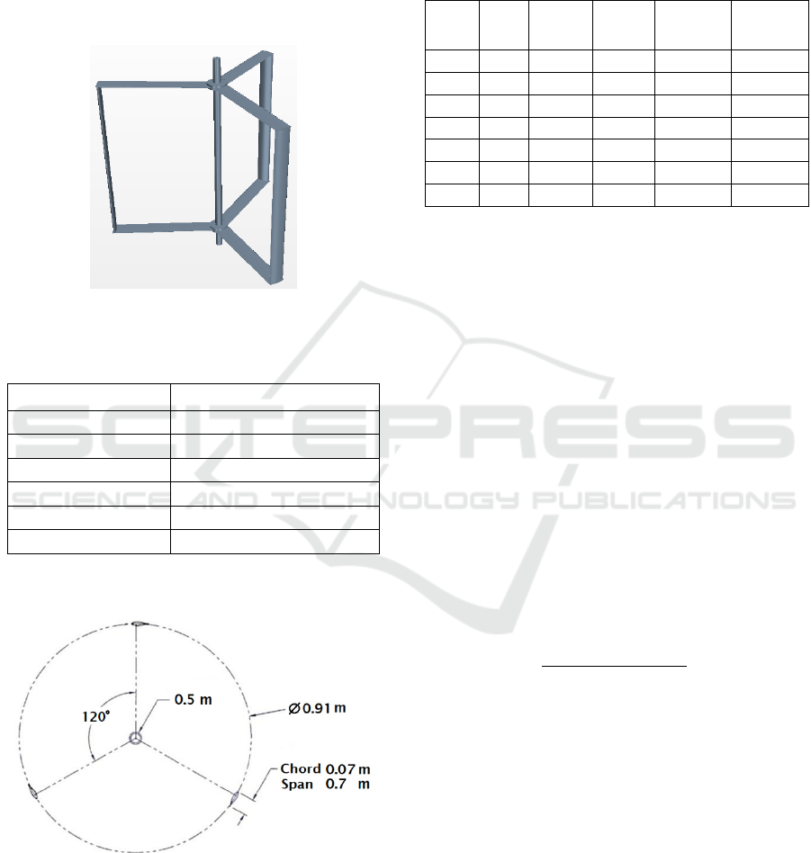
The turbine has diameter of 0.91 m, consists of 3

blades hydrofoil NACA 63(4)021 with chord 0.07 m

and span 0.7 m. The turbine geometry and

specifications can be seen in more detail in figure 1

and table 1.

Figure 1: Darrieus turbine geometry (Rawlings, 2008).

Table 1: Principal model turbine parameters (Rawlings,

2008).

Parameter Dimension and characteristic

Diamater turbine 0.91 m

Number of blades 3

Blade span 0.7 m

Blade profile NACA 63(4)021

Chord length 0.07 m

Shaft diameter 0.05 m

The turbine geometry in figure 1 can be shown in

the 2D sketch (top view) as shown in figure 2.

Figure 2: Turbine rotor sketch on top view (Rawlings,

2008).

3.2 Turbine Experimental Result

The turbine experimental data is reprocessed based

on the turbine performance graph. The experimental

result is processed using the turbine performance

formulations, as shown in point 2.2. Turbine

experiment data can be seen in table 2.

Table 2: Turbine experimental result (Rawlings, 2008;

reprocessed).

(m/s)

TSR

(rad/s)

(N.m)

(watt)

1.5 1.5 4.92 15.32 75.39 0.071

1.5 2.0 6.56 22.46 147.38 0.140

1.5 2.25 7.38 28.93 213.56 0.202

1.5 2.5 8.20 34.12 279.86 0.265

1.5 2.75 9.02 35.73 322.37 0.305

1.5 3.0 9.84 32.57 320.57 0.304

1.5 3.5 11.48 26.12 299.93 0.284

4 METHODOLOGY

The numerical simulation begins with creating

turbine geometry in .iges format. Next, the turbine

geometry is imported into the CFD program and

then creates boundary condition geometry and

region determination as domain modeling. For the

next step, generate grid meshing and do some

simulation settings such as selecting solver and input

initial condition and then running the simulation.

For validating the numerical modeling output

with the experimental result, firstly is to define the

boundary geometry dimension, and then study grid

meshing independency and compare the turbulence

model. The simulation is carried out with variating

TSR rate at constant current speed, 1.5 m/s.

Simulation result error is calculated using the

formulation:

% 𝑒𝑟𝑟𝑜𝑟=

𝑒𝑥𝑝𝑒𝑟𝑖𝑚𝑒𝑛𝑡−𝐶𝐹𝐷

𝑒𝑥𝑝𝑒𝑟𝑖𝑚𝑒𝑛𝑡

𝑥 100

(10)

To get the results of numerical modeling at a

certain degree of turbine rotation, the time step

calculation is required. Meanwhile, to determine a

total time for every single simulation, the physical

time calculation is required.

The time step in this study was calculated for

every 5° turbine revolute. While the physical time is

determined 10 times of the turbine rotation at the

current speed of 1.5 m/s.

Following is the example of calculating physical

time and time step at the turbine rotational speed of

4.92 rad/s.

Physical Time (for 10 times of turbine rotation)

can be calculated with the formulation:

ISOCEEN 2019 - The 7th International Seminar on Ocean and Coastal Engineering, Environmental and Natural Disaster Management

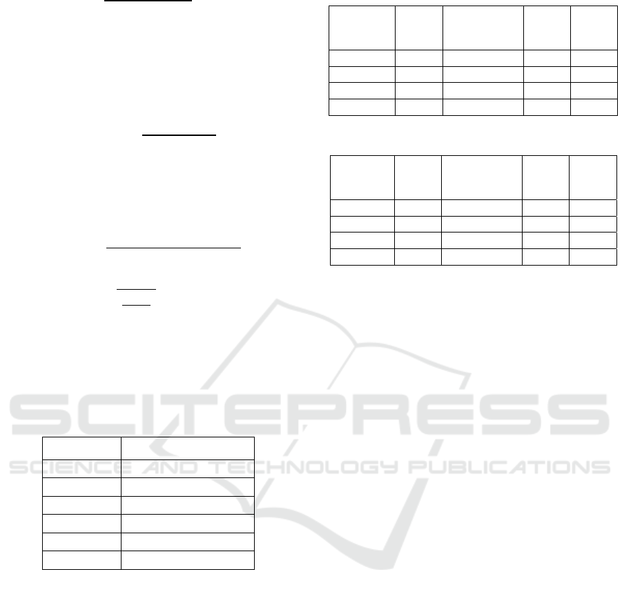
𝜔=

𝜃−𝜃



𝑃ℎ𝑦𝑠𝑖𝑐𝑎𝑙 𝑇𝑖𝑚𝑒

(11)

where :

𝜃 = degree for 1 rotation = 2𝜋 rad

𝜃



= degree for 0 rotation = 0

So that

𝑃ℎ𝑦𝑠𝑖𝑐𝑎𝑙 𝑇𝑖𝑚𝑒=

(

2𝜋− 0

)

𝑟𝑎𝑑

4.92 𝑟𝑎𝑑/𝑠

𝑥10

=12.8 𝑠

Time Step (for every 5° turbine revolute) can be

calculated with the formulation:

𝑇𝑖𝑚𝑒 𝑆𝑡𝑒𝑝=

𝑡𝑖𝑚𝑒

𝑓

𝑜𝑟 1 𝑠𝑖𝑚𝑢𝑙𝑎𝑡𝑖𝑜𝑛

𝑛𝑢𝑚𝑏𝑒𝑟 𝑜𝑓 𝑠𝑡𝑒𝑝𝑠

(12)

1.28 𝑠

(

360°

5°

)

=0.018 𝑠

The setting of the boundary condition domain in

every numerical simulation can be seen in table 3.

Table 3: Boundary condition domain in the numerical

modeling simulation.

Region Boundary condition

Inlet Uniform flow : 1.5 m/s

Outlet Pressure : 0 Pa

Side Walls Slip walls

Top Symmetry wall

Bottom Symmetry wall

Turbine Wall : no slip

5 RESULT AND DISCUSSION

5.1 Defining Boundary Geometry

Dimension

Numerical modeling uses 2D models so that the

determination of boundary sizes is sufficient to be

analyzed on the dimensions of length and width.

Simulation of defining boundary dimensions using

the same grid meshing composition, with input

current speed of 1.5 m/s and TSR 3.5.

The numerical simulation results based on

variations in boundary size can be seen in table 4

and table 5.

Table 4: Determination of boundary length.

Length

variations

(rad/s)

(experiment)

(CFD)

Error

L 12D 11.48 0.284 0.286 0.8%

L 14D 11.48 0.284 0.293 2.3%

L 16D 11.48 0.284 0.285 0.4%

L 18D 11.48 0.284 0.287 1.01%

Table 5: Determination of boundary width.

Width

variations

(rad/s)

(experiment)

(CFD)

Error

W 4D 11.48 0.284 0.45 59.3%

W 6D 11.48 0.284 0.34 19.4%

W 8D 11.48 0.284 0.29 0.4%

W 10D 11.48 0.284 0.28 2.8%

Based on the simulation results in table 4 and

table 5, the dimension of boundary condition

geometry is taken 12D in length and 8D in width,

where D is the turbine diameter.

5.2 Grid Independence Analysis

The independence grid study is conducted to define

the best grid composition for getting the best

analyzing results. There are several considerations

on the meshing process including the number of

grids generated, time for meshing, time for

simulating, the computer performance and the error

value.

In the analysis of grid independence, the

simulations are carried out with variation number of

grid. Figure 3 shows grid meshing comparison

between tenuous and precision density. For the next,

to find out the numerical results based on the

number of grid density, this study simulates Darrieus

turbine on the current velocity of 1.5 m/s and TSR

3.0. The simulation results are presented in table 6.

The simulation result in table 6 shows that the

numerical model with the smallest error value is

produced when using meshing 5. However,

consideration to the computer performance which

difficult to generate meshing 9,207,251 cells and

need longer time for simulation, so that it is decided

to use meshing 4 with error value 3.3%. This error

value is not much different from the error value of

meshing 5. Moreover, meshing 4 only consists of

73,397 cells after being converted into the 2D

model.

Numerical Modeling of Vertical Axis Hydro Turbine with Experimental Validation

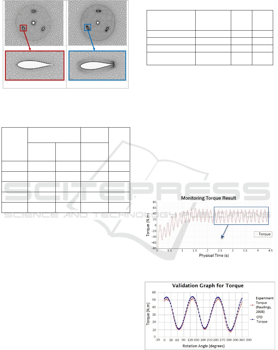
Figure 3: Comparison of meshing results when using

tenuous grid (a) and precision grid (b).

Table 6: Numerical simulation results based on number

grids variations.

Meshing

variations

Grids number

Time for

simulation

Error

Model 3D

Covert to

(minutes)

Meshing 1 1,387,775 66,410 38 20.4%

Meshing 2 2,546,383 68,619 45 18.5%

Meshing 3 3,944,757 71,394 75 15.2%

Meshing 4 6,107,915 73,397 96 3.3%

Meshing 5 9,207,251 78,295 135 0.8%

5.3 Turbulence Model Comparison

One of the factors that have a great effect on the

result of the CFD analysis is the flow turbulence

model. The numerical validation process in this

study simulates several turbulence models to define

what turbulence model produces the smallest error

values. The turbulence models that compared in this

study are k-ε, k-ω SST, Spalart Allmaras and

Reynolds Stress Turbulence.

Turbulence model comparison is performed at

the current velocity of 1.5 m/s, TSR 2.5, and using

the turbulence intensity of 0.05 (Marsh, 2015,2016).

The simulation result of the turbulence model

comparison can be seen in table 7.

The simulation result in table 7 shows that the

smallest error is produced by k-ω SST turbulence

model. This result has corresponded with many

studies (Dai, 2009; Marsh, 2015; 2016; Castelli,

2010; Rahmawati, 2017; Nobile, 2011; Madi, et.al.,

2019) who used the k-ω SST model in their ocean

current turbine numerical model.

Table 7: The result of turbulence model comparison.

Turbulence Models

(experiment)

(N.m)

(CFD)

(N.m)

Error

k- ε 34.12 38.11 11.7%

k-ω SST 34.12 36.67 7.5%

Spalart Allmaras 34.12 39.42 15.5%

Reynolds Stress

Turbulance

34.12 26.62 22%

5.4 Numerical Validation Result

After defining boundary geometry dimensions, grid

independency analysis, and selecting the turbulence

model appropriate, then the next step is validation

the numerical model of Darrieus turbine with the

experimental result. The validation parameter is the

torque that correlates with the performance

coefficient.

5.4.1 Torque Validation

Torque simulation for the validation process is

performed at the current speed of 2 m/s and TSR

2.5. The result of torque using numerical model

CFD is shown in figure 4 and validation with the

experimental result is shown in figure 5.

Figure 4: Torque result of numerical modeling at the

current speed of 2 m/s and TSR 2.5.

Figure 5: Torque validation at the current speed of 2 m/s

and TSR 2.5 for 1 rotation.

The avera

e tor

ue value is calculated in the last 5 rotations

(a) Volume mesh 2,546,383 cells

(b) Volume mesh 6,107,915 cells

ISOCEEN 2019 - The 7th International Seminar on Ocean and Coastal Engineering, Environmental and Natural Disaster Management

One of the torque validation can be seen in figure

5. On the figure, both experimental torque and CFD

torque are simulated at the current speed of 2 m/s

and TSR 2.5. The validation torque on this condition

has error value of 7.02%.

5.4.2 Coefficient of Performance (Cp)

Validation

The coefficient of performance well known as

turbine efficiency is the ratio between power

produced by the turbine operating with the potential

current energy absorbed by the turbine theoretically.

Turbine efficiency and its validation can be

calculated using several data such as turbine

dimension, current velocity and torque result both

from experimental testing and CFD analysis.

For example, turbine efficiency and its validation

are calculated at the current speed of 1.5 m/s, TSR

1.5.

Using equation 8, the theoretical power potential

of the turbine can be calculated

Pt = 0.5 x 1000 kg/m3 x (0.91 m x 0.7 m) x

(1.5 m/s)3 = 1055.64 watt

Using equation 7, the turbine power from CFD

analysis can be calculated.

PnCFD = 4.92 rad/s x 16.59 N.m

= 81.65 watt

The result of turbine efficiency from CFD analysis

can be calculated using equation 6.

CpCFD = 81.65 watt / 1055.64 watt

= 0.077

By using the experimental data in table 2, the

validation of turbine efficiency can be calculated

using equation 10.

% error = ([0.071-0.077] / 0.07) x 100

= 8.3 %

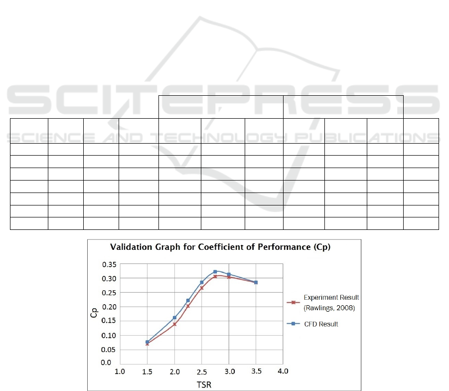
The validation results of CFD analysis and

experimental data of turbine Darrieus can be seen in

detail in table 8 and figure 6.

Table 8 shows the comparison between the CFD

analysis and the experimental results. CFD analysis

uses initial conditions which are equated with

Table 8: The validation of Darrieus turbine numerical CFD and experimental results.

Experimental result

(Rawlings, 2008; reprocessed)

Numerical CFD

m/s

TSR

(rad/s)

(watt)

(N.m)

(watt)

(N.m)

(watt)

Cp Error

1.5 1.5 4.92 1055.64 15.32 75.39 0.071 16.59 81.65 0.077 8.3%

1.5 2.0 6.56 1055.64 22.46 147.38 0.140 26.17 171.70 0.163 16.5%

1.5 2.25 7.38 1055.64 28.93 213.56 0.202 31.73 234.21 0.222 9.7%

1.5 2.5 8.20 1055.64 34.12 279.86 0.265 36.67 300.77 0.285 7.5%

1.5 2.75 9.02 1055.64 35.73 322.37 0.305 37.64 339.62 0.322 5.4%

1.5 3.0 9.84 1055.64 32.57 320.57 0.304 33.63 330.98 0.314 3.3%

1.5 3.5 11.48 1055.64 26.12 299.93 0.284 26.23 301.23 0.285 0.4%

Figure 6: Darrieus turbine performance on numerical CFD and experimental results.

Numerical Modeling of Vertical Axis Hydro Turbine with Experimental Validation

experimental data that are simulated at the current

speed of 1.5 m/s with TSR variations between 1.5 to

3.5. Validation results are obtained numerical model

error value at TSR 1.5 is 8.3%, TSR 2.0 is 16.5%,

TSR 2.25 is 9.7%, TSR 2.5 is 7.5%, TSR 2.75 is

5.4%, TSR 3.0 is 3.3%, and at TSR 3.5 is 0.4%.

Figure 6 shows that the Cp of the CFD analysis

results tend to be higher than the Cp of the

experimental results because numerical analysis uses

2D models that ignore the influence of the turbine

arm in the simulation. Basically the turbine arm will

produce a drag force which can reduce turbine

performance.

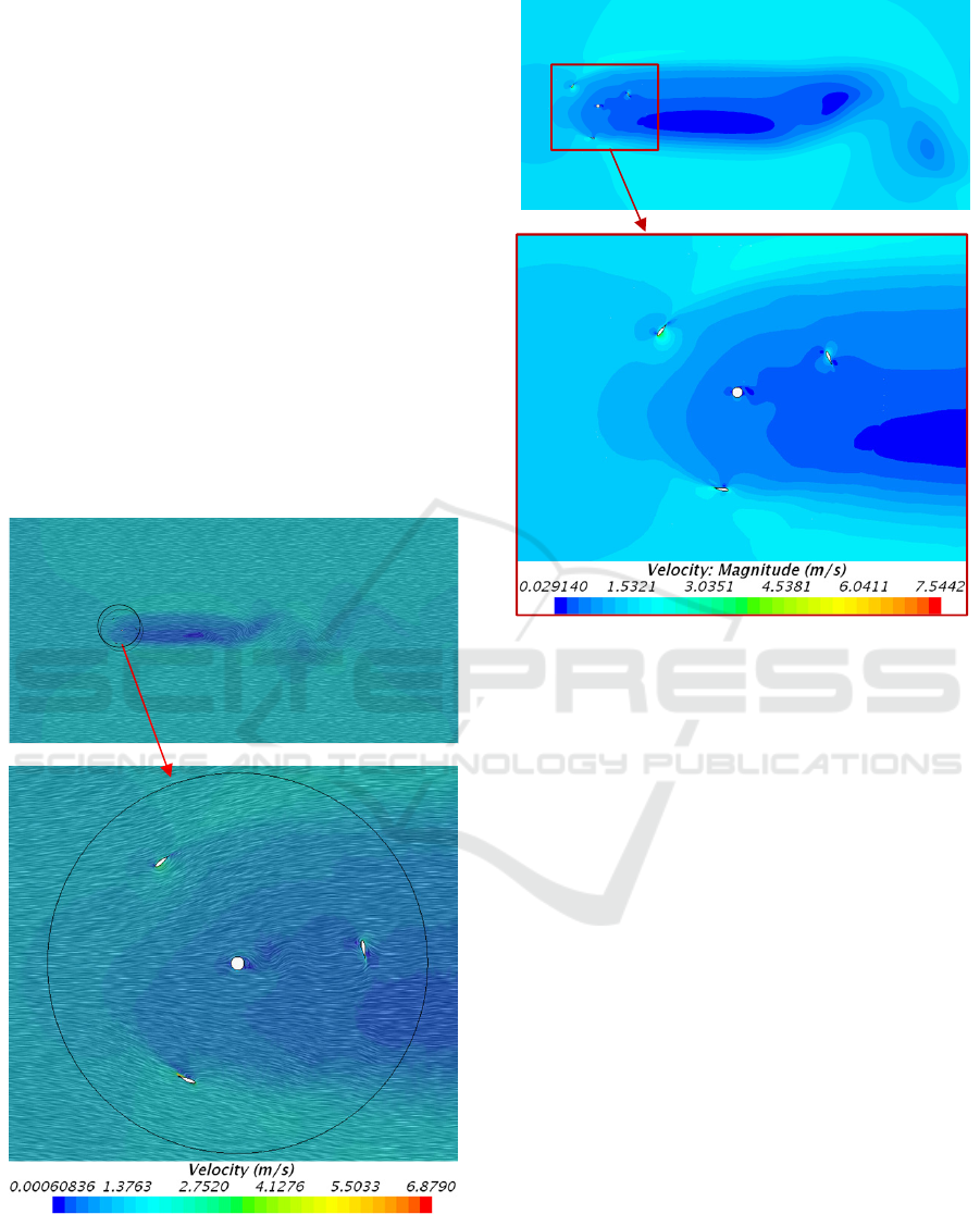
The numerical modeling results of the Darrieus

turbine are presented in the flow direction vector

that trought pass the turbine and flow velocity

contour as shown in figures 7 and 8. In these figures,

the Darrieus turbine is simulated at the free stream

speed of 1.5 m/s with TSR 2.75 (figure 7) and TSR

3.5 (figure 8).

Figure 7: Flow velocity direction on the turbine, rotating at

TSR 2.75.

Figure 8: Flow velocity contour on the turbine, rotating at

TSR 3.5.

6 CONCLUSION

Validation of the Darrieus turbine numerical model

starts from defining the boundary geometry

dimension, study the grid independency, and

selecting the turbulence model appropriate. The

numerical modeling error value at TSR 1.5 is 8.3%,

TSR 2.0 is 16.5%, TSR 2.25 is 9.7%, TSR 2.5 is

7.5%, TSR 2.75 is 5.4%, TSR 3.0 is 3.3%, and at

TSR 3.5 is 0.4%. The average error is 7.3% which is

categorized as a good agreement result.

ACKNOWLEDGMENTS

A great appreciation to supervisors and all members

of Marine Engineering Postgraduate Laboratorium,

Sepuluh Nopember Institut of Technology Surabaya

for support throughout the project. Authors also

would like to thanks all colleagues from Agency for

the Assessment and Application of Technology

(BPPT) especially the work unit of Center of

Technology for Maritime Industrial (PTRIM) and

ISOCEEN 2019 - The 7th International Seminar on Ocean and Coastal Engineering, Environmental and Natural Disaster Management

Hydrodynamic Institute of Technology (BTH) for

providing facility and supporting the project.

REFERENCES

Castelli, M. R., Ardizzon, G., Battisti, L., Benini, E.,

Pavesi, G., 2010. Modeling Strategy and Numerical

Validation for a Darrieus Vertical Axis Micro-wind

Turbine. In International Mechanical Engineering

Congress and Exposition. ASME.

Dai, Y. M., Lam, W., 2009. Numerical Study of Straight-

bladed Darrieus-type Tidal Turbine. In ICE-Energy;

162:67-76.

Daruwedho, H., Sasmito, B., Janu, A. F., 2016. Analysis

of Sea Surface Levels in Indonesian Waters Using the

Jason-2 Altimetry Satellite 2010-2014 (in Indonesian

language). In Jurnal Geodesi Undip; 5(2):145-158.

Hantoro, R., Prananda, J., Mahmashani, A. W.,

Septyaningru, E., and Imanuddin, E., 2018.

Performance Investigation of an Innovative Vertical

Axis Hydrokinetic Turbine-Straight Blade Cascaded

(VAHT-SBC) for Low Current Speed. In Journal of

Physics; 1022: 1-8. IOP Publishing.

Hantoro, R., Utama, I. K. A. P., Erwandi, Sulisetyono, A.,

2009. Force Instability and Fluid-Structure Interaction

in Vertical Axis Turbines for Generating Tidal Current

Energy (in Indonesian language). In Jurnal Teknik

Mesin; 11(1):25-33.

Hantoro, R., Utama, I. K. A. P., Erwandi, Sulisetyono, A.,

2011. An Experimental Investigation of Passive

Variable-Pitch Vertical-Axis Ocean Current Turbine.

In ITB J Eng Sci; 43(1):27-40.

Kasharjanto, A., Rahuna, D., Aditya, R. B., 2017. Test

Performance of Tidal Current Turbine 10 Kilowatt

using Double Hull Platform on the Suramadu Bridge

(in Indonesian language). In Jurnal Ilmu Pengetahuan

& Teknologi Kelautan; 14:79-86.

Madi, Sasono, M. E. N., Hadiwidodo, Y. S., Sujiatanti, S.

H., 2019. Application of Savonius Turbine behind The

Propeller as Energy Source of Fishing Vessel in

Indonesia. In IOP Conference Series: Materials

Science and Engineering. IOP Publishing.

Marsh, P., Ranmuthugala, D., Penesis, I., Thomas, G.,

2015. Numerical Investigation of the Influence of

Blade Helicity on the Performance Characteristics of

Vertical Axis Tidal Turbines. In Renewable Energy;

81:926-935.ELSEVIER.

Marsh, P., Ranmuthugala, D., Penesis, I., Thomas, G.,

2015. Three-Dimensional Numerical Simulations of

Straight-bladed Vertical Axis Tidal Turbines

Investigating Power Output, Torque Ripple and

Mounting Forces. In Renewable Energy; 81:67-77.

ELSEVIER.

Marsh, P., Ranmuthugala, D., Penesis, I., Thomas, G.,

2016. Numerical Simulation of the Loading

Characteristics of Straight and Helical-bladed Vertical

Axis Tidal Turbines. In Renewable Energy; 94:418-

428. ELSEVIER.

MeyGen, 2019. SSIMEC Atlantis Energy. In

https://simecatlantis.com/projects/meygen. (accessed

on 17 October 2019).

Mukhtasor, Susilohadi, Erwandi, Pandoe, W., Iswadi, A.,

Firdaus, A. M., Prabowo, H., Sudjono, E., Prasetyo,

E., and Ilahude, D., 2014. Ocean Energy Resources in

Indonesia (in Indonesian language). Marine

Geological Research and Development Center (P3GL)

Ministry of Energy and Mineral Resources,

Association of Marine Energy of Indonesia (ASELI).

Mulualem, 2012. Simplified CFD Modelling of Tidal

Turbines for Exploring Arrays of Devices. Thesis PhD.

University of Exeter.

Nobile, R., Vahdati, M., Barlow, J. F., Mewburn-Crook,

A., 2011. Dynamic Stall for a Vertical Axis Wind

Turbine in a Two-Dimensional Study. In World

Renewable Energy Congress: 4225-4232.

LINKÖPINGS UNIVERSITET.

Rachmat, B., and Ilahude, D., 2015. Determining Location

of Tidal Current Turbine Power Plant-Small Scale in

Liatung Starit, Talaud, North Sulawesi (in Indonesian

language). In Jurnal Geologi Kelautan; 13(3):127-

142.

Rahmawati, S., 2017. Study on Characteristics of Tidal

Current Energy and Ocean Environmental Pollution

at Indonesia Archipelago. Doctor Dissertation.

Hiroshima University.

Rawlings, G. W., 2008. Parametric Characterization of an

Experimental Vertical Axis Hydro Turbine, Thesis,

Faculty of Graduate Studies (Mechanical

Engineering): University of British Columbia,

Vancouver.

Salim, M., Buccolieri, R., Chan, A., Sabatino, S., 2011.

Numerical Simulation of Atmospheric Pollutant

Dispersion in an Urban Street Canyon: Comparison

Between RANS and LES. In Journal of Wind

Engineering and Industrial Aerodynamics; 99(2):103-

113. ELSEVIER.

Sun, X., Chick, J., Bryden, G., 2008. Laboratory-scale

Simulation of Energy Extraction From Tidal Currents.

In Renewable Energy; 33(6):1267-1274. ELSEVIER.

Numerical Modeling of Vertical Axis Hydro Turbine with Experimental Validation