Plug and Play Deep Convolutional Neural Networks

Patrick Neary and Vicki Allan

Department of Computer Science, Utah State University, Old Main Hill, Logan, U.S.A.

Keywords:

Image Recognition, Machine Learning, Convolutional Neural Networks, Artiﬁcial Intelligence, Hyperparam-

eter Tuning, Deep Learning.

Abstract:

Major gains have been made in recent years in object recognition due to advances in deep convolutional neural

networks. One struggle with deep learning is identifying an optimal network architecture for a given problem.

Often different conﬁgurations are tried until one is identiﬁed that gives acceptable results. This paper proposes

an asynchronous learning algorithm that ﬁnds an optimal network conﬁguration by automatically adjusting

network hyperparameters.

1 INTRODUCTION

There are a variety of neural network structures that

are commonly used in industry and research. Con-

volutional neural networks (CNNs) are a favorite for

image recognition tasks. CNNs have been constructed

using different components. One predominant archi-

tecture uses four building blocks: convolutional lay-

ers, pooling, normalization, fully connected layers,

and activation functions. A major consideration in

CNN design is the number and conﬁguration of each

of the aforementioned components. A network is of-

ten considered ‘deep’ when it has more than two of

these layers.

Numerous applications use CNNs in image recog-

nition. Much of the success achieved in this area is

due to deep neural networks (LeCun et al., 2015).

While deep networks have enabled many interesting

and useful applications, a number of hurdles remain

to be overcome. One hurdle is the fact that, as of

yet, there is not an analytic way to determine the opti-

mal architecture for solving speciﬁc problems. Often

researchers create several different network architec-

tures and then select the best one for their applica-

tion ((Schwegmann et al., 2016), (Chen et al., 2016),

(Wang et al., 2017), and (Pu et al., 2016)). Manually

creating architectures and training them can be a time

consuming and laborious process.

One of the challenges in working with neural net-

works is selecting an ideal architecture for a given

task. Currently, to the authors’ knowledge, there is

not a standard approach to building an optimal net-

work conﬁguration. There are different neural net-

work types, and each one has a variety of hyperpa-

rameters that can be adjusted. In this work, ﬁlter di-

mensions, number of ﬁlters, number of convolutional

layers, number of fully connected layer nodes, num-

ber of fully connected layers, presence of pooling and

normalization are tuned.

Knowledge regarding the science and the art of

parameter tuning for CNNs is required to be suc-

cessful using CNNs. This paper proposes an auto-

mated approach to tuning hyperparameters that gives

the layman and professional alike the ability to gen-

erate CNN architectures which are built and trained

from scratch on their data. We will refer to the algo-

rithm in this paper as ‘Plug and Play’ (PnP) to differ-

entiate it from other algorithms.

2 PREVIOUS WORK

Hyperparameter tuning is not a new problem. (Le-

Cun et al., 1998) discussed the issue back in 1998. It

is well known that architectures play a role in deter-

mining the difference between competitive and non-

competitive results (Domhan et al., 2015).

Early approaches to the hyperparameter dilemma

include a grid space search (LeCun et al., 1998). In

grid space search, upper bounds, lower bounds, and

step size are established for hyperparameters of inter-

est. The algorithm then steps through conﬁgurations

in the grid search. If step sizes are too big, the best

conﬁgurations may be skipped. The smaller the step

sizes are, however, the longer it takes to run through

the possible combinations of parameters. The number

388

Neary, P. and Allan, V.

Plug and Play Deep Convolutional Neural Networks.

DOI: 10.5220/0007255103880395

In Proceedings of the 11th International Conference on Agents and Artiﬁcial Intelligence (ICAART 2019), pages 388-395

ISBN: 978-989-758-350-6

of conﬁgurations to test, increases exponentially with

the number of hyperparameter discrete states (Koch

et al., 2018).

Upon completion of the grid search, the best con-

ﬁguration is selected. Problems with the grid search

include spending too much time training spaces that

are known to be irrelevant, and not enough empha-

sis on areas that are of high interest. For example, it

may be the case that increasing the number of neu-

rons in a fully connected layer above 2048, does not

add any beneﬁt. It also may be that using less that 512

neurons per layer produces sub-optimal results. With

a grid search these extremes continue to be explored

despite the fact that they produce bad results or do not

add any beneﬁt.

The approach proposed in this paper is different

from grid search, in part, because it uses correlations

and a binary search method to traverse and identify

the best performing parameter values.

A subsequent approach is random search

(Bergstra and Bengio, 2012). Lower and upper

bounds have to be speciﬁed for the random search

and then it will randomly sample the parameter

search space. Upon completion, the best conﬁgura-

tion is selected. In practice, a second search is often

performed in the local region of the best performing

conﬁguration. Random search has been found to be

superior to grid search in a variety of applications.

(Bergstra and Bengio, 2012) demonstrated that

random search works better than grid search.

The reason that random search is believed to per-

form better than grid search is because random search

is granted the same computational budget, but is al-

lowed to randomly explore a wider range of conﬁg-

urations. It also is not limited to ﬁxed stepped in-

crements between upper and lower hyperparameter

bounds, like within a grid search. Due to the increased

range of hyperparameter values, it is able to ﬁnd con-

ﬁgurations that would have otherwise been impossi-

ble, due to upper and lower bounds of the grid search.

However, it is still possible that the ideal combina-

tion of hyperparameter settings is overlooked because

that combination of parameters is not in the randomly

sampled set (Koch et al., 2018).

Another approach to hyperparameter tuning uti-

lizes Bayesian methods. For example, Sequential

Model-based Algorithm Conﬁguration (SMAC) (Hut-

ter et al., 2011) uses probability models to correlate

hyper-parameters to the loss function. Tree-structured

Parzen Estimator (TPE) (Bergstra et al., 2011) uses

a set of models that effectively track hyperparameter

values that perform well versus those that do not. It

makes decisions regarding how to build the network

architecture based on the models it builds internally.

The grid and random search approaches are attrac-

tive and are used in practice due to their simplicity

(Bergstra and Bengio, 2012). SMAC and TPE are

also used and give good results, but are more com-

plex to implement. All of these approaches require

substantial time to run, and require the practitioner to

provide hyperparameter limits.

Autotune (Koch et al., 2018) is another recent

method for hyperparameter tuning. This algorithm

takes a collection of hyperparameter tuning methods

(Bayesian, random, genetic, DIRECT, etc.) and runs

them in parallel. Information generated from each

method is recorded and used as the collection of algo-

rithms are run. Their tests used 40 parallel compute

nodes and completed their training in a day. Assum-

ing a direct translation from parallel to serial compu-

tation, this approach would take 40 days on a single

compute node. Autotune was built for SAS



Other efforts have been made to algorithmically

learn optimal network architectures. For example,

(Baker et al., 2016) used a reinforcement learning

based approach. While they were able to achieve

good results, it came at the cost of a signiﬁcant

amount of training time. For example, it took an aver-

age of 8-10 days to train the ﬁrst iteration of their al-

gorithm and then additional time to ﬁne tune the train-

ing for subsequent stages. The training took place on

a high end system containing 8 GPUs.

We propose a competing algorithm to the afore-

mentioned approaches that is simple in principle and

in application, while yielding competitive results. In

addition, our approach relieves the user from the bur-

den of determining upper and lower hyperparameter

bounds, learning rates, and other initialization con-

straints. Some hyperparameter tuning algorithms go

through the process of adjusting hyperparameters, but

still leave optimization of learning rates to the user

when the algorithm has completed (Hinz et al., 2018).

Our work handles learning rates as well. The resulting

algorithm can be pointed at a directory of categorized

images and it produces an optimized network archi-

tecture that can be used for their end goals.

3 BACKGROUND

A number of hyperparameters need to be selected

carefully in order to: keep weights from diverging,

ensure quick convergence and achieve optimal results.

These include selecting the learning rate, weight ini-

tialization, and activation function selection.

Plug and Play Deep Convolutional Neural Networks

389

3.0.1 Convolutional Neural Networks

In the context of neural networks, a convolution is a

mathematical operation applied to data presented to

the network. Convolutions are able to take advan-

tage of the two dimensional information in images.

Convolving ﬁlters with images allows characteristics,

such as lines and shapes, to be extracted from the im-

age. This information is used to identify objects. Con-

volutional neural networks are often used with im-

agery.

3.0.2 Learning Rates

Many neural networks use gradient descent to update

weights. α, in equation 1, is the learning rate, θ is

a weight, and ‘J’ is the cost function of θ. If the

learning rate is too small, then gradient descent can

be very slow. If it is too large, then the solution will

likely diverge. The best learning rate generally varies

from one architecture and data set to the next because

the dynamics of each is unique.

θ = θ − α

dθ

J(θ) (1)

One area of research has focused on how to set

learning rates. In practice, several different learning

rates are tried and the one with the best results is

used. Another common practice is to adjust learning

rates following an exponential decay curve. (Smith,

2017) found that adjusting the learning rate in a trian-

gle waveform (cyclic learning rate) produces excep-

tional results.

3.0.3 Weights

CNNs require weights to be initialized. Weights, im-

properly initialized, can yield vanishing gradients or

result in symmetry between hidden units in a given

layer. A standard approach for initializing weights is

to use a Gaussian distribution with 0.01 standard de-

viation.

An improvement on this approach is the ‘Xavier’

method suggested in (Glorot and Bengio, 2010). This

method uses equation 2 to generate weights, where

is the number of inputs coming into the neuron

and n

out

is the number of neuron outputs to the next

layer. ‘Var’ is the variance to be applied to the neuron

weights, ‘W’, when initialized. This allows weight

initialization to vary appropriately with network con-

ﬁguration.

Var(W ) = 2

+ n

out

(2)

3.0.4 Activation Functions

Rectiﬁed linear unit (ReLU) activation functions

have been critical in enabling deep network success

(Krizhevsky et al., 2017). One problem with ReLU

activation functions is that they may die at zero dur-

ing training, subsequently leaving the node worthless.

A signiﬁcant solution to this problem is the Paramet-

ric Rectiﬁed Linear Unit (PReLU) (He et al., 2015)

which allows negative values rather than bottoming

out at zero.

3.0.5 Filters

Each individual ﬁlter is tuned to pull out speciﬁc fea-

tures in an image. For example, ﬁlters may identify

horizontal and vertical features in an image. Gener-

ally, deeper layers are able to identify more complex

patterns and objects within an image.

It is not always known beforehand how many ﬁl-

ters are needed to identify features of interest in a data

set. This research explores setting these values algo-

rithmically, thus saving time for the practitioner. The

algorithm explores the space of options based on cor-

relations between parameter settings and resulting ac-

curacy.

3.0.6 Pooling

There are a wide variety of ways to modify convo-

lutional neural network architectures. Two common

operations are pooling (Scherer et al., 2010) and nor-

malization (Ioffe and Szegedy, 2015).

Pooling is a process that helps reduce data dimen-

sions in the convolutional neural network. Gener-

ally, when pooling is applied, a 2x2 mask is used to

slide over every product that comes out of a convo-

lutional layer. In max pooling, for example, the 2x2

mask is moved over the data and the maximum value

from the area under the mask is passed to the output.

Similarly, average pooling will take the average value

of the masked area and use it to create a new two-

dimensional data set.

3.0.7 Normalization

Another common operation is layer normalization.

Layer normalization is a process where inputs to neu-

rons in a layer are normalized. It is performed by us-

ing Equation 3, where ¯x is calculated from all inputs

to neurons in the current layer for a single instance.

The purpose of normalization is to help with vanish-

ing and exploding gradients.

ˆx =

x − mean(¯x)

std( ¯x)

(3)

ICAART 2019 - 11th International Conference on Agents and Artiﬁcial Intelligence

390

3.0.8 Fully Connected Layer

On the output of the last convolutional layer, there is

often a fully connected network. More than one fully

connected layer (FCL) may be present. FCLs have

the role of identifying patterns and predicting results.

FCLs can take on any number of layers and any num-

ber of perceptrons in each layer.

This work introduces an asynchronous approach

to methodically move through network architectures.

The algorithm settles on an architecture that gives

competitive performance. All the user has to do is

point the algorithm at a directory of images and press

the ‘go’ button. When the algorithm has ﬁnished run-

ning, a network architecture is ready that can give

great results.

The contributions of this paper include the fol-

lowing. Bringing together disparate algorithms into

a cohesive approach for automatically tuning hy-

perparameters. Speciﬁcally, the algorithm identi-

ﬁes optimal network weight distributions and maxi-

mum/minimum learning rates unique to each network

architecture. The algorithm moves through various

architectures in an asynchronous fashion. In the end,

a network architecture with corresponding weights is

produced in a format that can be directly applied by

the end user. This is accomplished in much less time

than competing methods. The user does not need to

provide upper or lower limits for any of the hyperpa-

rameters.

4 METHODOLOGY

While the tuning algorithm is running, training takes

place long enough to determine whether the changes

have produced favorable results or not. Once the al-

gorithm has completed, the training is allowed to con-

tinue for a longer period of time to generate ﬁnal re-

sults.

From a high level, the current tuning algorithm

works through the convolutional layers ﬁrst, followed

by the fully connected layers. One of the fundamen-

tal ideas in this hyperparameter tuning algorithm is to

identify the correlation between accuracy and the di-

rection that parameters are adjusted. This correlation

is used to direct the adjustment of the hyperparameter.

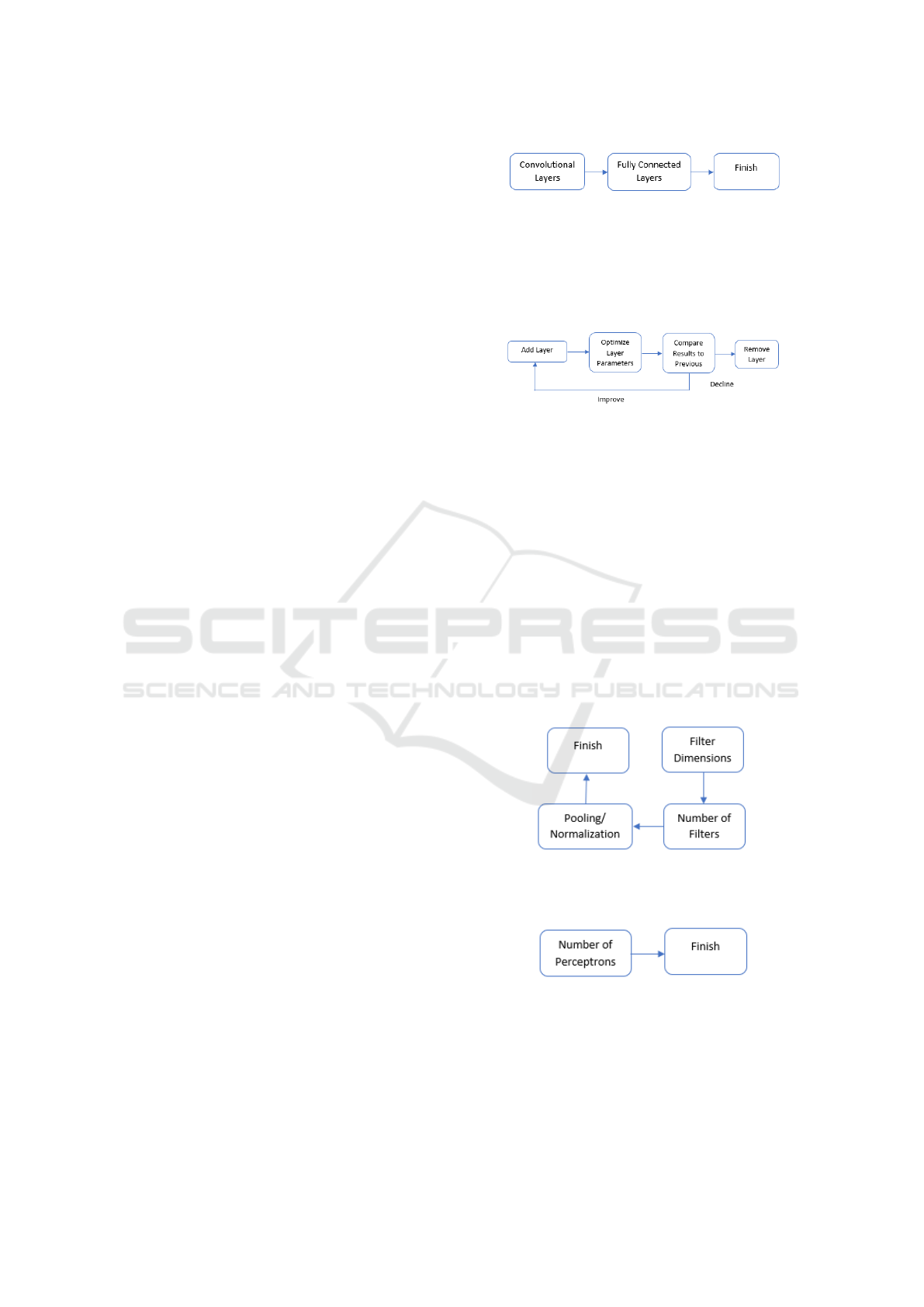
Figure 1 displays the high level convolution layer

tuning process. It shows that the convolution layers

are ﬁrst tuned, followed by the fully connected layers.

Figure 2 shows the process undergone in both

the convolutional and fully connected layers. A new

layer is added, relevant hyperparameters are tuned,

and then results are compared to previous results. If

Figure 1: High level approach to tuning. Convolution layers

are ﬁrst tuned, followed by fully connected layers.

there is an improvement, another layer is added and

the process is repeated. If the results degrade, then

the layer causing the degradation is dropped, and then

the loop exits.

Figure 2: Tuning for convolution layers. Layers are added

one at a time according to this process.

For tuning hyperparameters in the convolution

layers, the process in Figure 3 is followed. Figure

3 represents the “Optimize Layer Parameters” block

in Figure 1. Filter dimensions, number of ﬁlters, and

pooling/normalization are evaluated in sequence. In

the example of ﬁlter dimensions, three different di-

mensions are evaluated. The resulting accuracies are

evaluated and a correlation is calculated. Once the di-

rection to change parameters is determined, a binary

search is used to identify the best performing hyper-

parameter value. Once the number of ﬁlters have been

set, pooling and normalization are applied to see if

they improve the overall performance of the layer. If

not, they are removed.

Figure 3: Tuning for a single convolution layer. Hyperpa-

rameters for each layer are tuned before moving on to the

next layer.

Figure 4: Fully connected layer tuning. The number of neu-

rons is optimized, layer by layer, in the fully connected por-

tion of the network.

The fully connected layers currently have two pa-

rameters of interest, the number of fully connected

layers and the number of perceptrons in each layer.

Figure 4 represents the “Optimize Layer Parameters”

Plug and Play Deep Convolutional Neural Networks

391

block in Figure 1. Correlations are used to determine

the direction to adjust the parameter, followed by a

binary search for the best performing value. When

there is a degradation in ﬁnal results, the current layer

is removed and the previous conﬁguration is used.

With the high level algorithm established, we will

discuss how each hyperparameter is selected in more

detail.

To identify the best ﬁlter dimensions, ﬁve asyn-

chronous training agents are launched. Each agent

trains a conﬁguration where everything but the ﬁlter

dimensions are kept constant. As each agent com-

pletes, it returns the training accuracy. The new train-

ing accuracies are compared and the ﬁlter dimension

that yields the best results is returned to the main

agent.

After optimizing ﬁlter dimensions, the number of

ﬁlters for the current convolution layer is identiﬁed.

Again, asynchronous training agents are launched,

each one with a unique number of ﬁlters while all

other hyperparameters are kept constant. The ﬁlter

conﬁguration that produces the best accuracy is re-

turned to the master process.

With the number of ﬁlters and their dimensions

ﬁxed, the fully connected layer conﬁguration is ex-

plored next. To identify the best conﬁguration for

the ﬁrst layer, asynchronous agents are spawned that

identify the best number of nodes for the ﬁrst fully

connected layer. Next, a new fully connected layer

is added, and a new set of asynchronous agents are

spawned. Additional fully connected layers are added

until improvement in accuracy drops. When accuracy

drops, the most recently added layer is dropped, the

algorithm terminates, and the resulting network archi-

tecture is saved.

Each time a new architecture is created as previ-

ously described, the system identiﬁes the maximum

and minimum learning rates. Each iteration requires

identifying the maximum and minimum because each

conﬁguration has different dynamics than the last.

Additionally, cyclic learning rates are used in the pat-

tern established by (Smith, 2017).

5 RESULTS

In this section we discuss conﬁguration details for the

experiments and the subsequent results.

5.1 Experimental Setup

While many interesting data sets exist, most compara-

ble hyperparameter tuning algorithms that have been

published, work with MNIST and CIFAR-10. Due to

the broad support of these two data sets, this work will

also use them to compare results against other estab-

lished methods.

The MNIST and CIFAR-10 data sets each have

60,000 images. The sets partition 50,000 images for

training and validation, while 10,000 images are re-

served for testing. From the set of 50,000 images,

75% of the data is used for training and 25% is used

for validation. All images are organized into a folder

structure where each image class is contained in a

sub-directory.

Training was performed on a Windows laptop

with 8 CPU cores and an NVIDIA GeForce GPU.

For this research the following hyperparameters are

adjusted: number of weights, learning rates, convolu-

tional layers, number of ﬁlters per layer, size of the

kernels, number of fully connected layers, and num-

ber of neurons in each fully connected layer. The cost

calculation is based on a softmax cross entropy func-

tion.

As a starting point, the algorithm uses the param-

eters outlined in Table 1.

Table 1: Starting hyperparameter conﬁguration. Hyperpa-

rameter values are listed, along with the starting value and

the amount by which the parameters can change.

Hyperparameter Start Val Inc Val

Filter Dimensions 3x3 1x1

Number of Filters 32 32

Convolution Layers 1 1

Fully Connected Layers 1 1

Neurons per FCL 32 32

While there are a variety of activation functions

to choose from, we chose to use PReLu for reasons

discussed in Section 3.

There are also a variety of optimization algorithms

to use in training. Rather than using gradient descent,

we use the Adam Optimizer (Kingma and Ba, 2014)

for training. Adam provides faster convergence in

training than gradient descent and is, consequently, a

good selection for hyperparameter tuning.

When CNNs are created in this work, weights are

initialized using the Xavier methodology (Glorot and

Bengio, 2010).

5.2 Experiment Results

The methodology section discussed the approach

taken to optimize hyperparameters. Each convolution

layer is built up sequentially starting with the number

of ﬁlters followed by the ﬁlter dimensions. Training at

each level happens with asynchronous agents that re-

turn their results to the master agent. Each agent starts

ICAART 2019 - 11th International Conference on Agents and Artiﬁcial Intelligence

392

by identifying the maximum learning rate to use and

then employs a decreasing maximum cyclic learning

rate during training. Once the convolution layers have

converged to the maximum extent possible, the fully

connected layers are then adjusted cyclically.

The learning agents are allowed to run through the

hyperparameters as previously discussed. The algo-

rithm achieves an accuracy of 99.1% for the optimal

result for the available range of hyperparameters for

the MNIST data set.

Table 2 shows convergence of the MNIST data set

using this algorithm. For entries in the ‘Filter Dimen-

sions’ column, the list on each row shows the ﬁnal

ﬁlter dimensions selected for each convolution layer.

[[5, 5], [5, 5]], for example, indicates that the ﬁrst

and second convolution layer ﬁlters have dimensions

of 5x5. Each entry in the ‘Filters’ column shows the

number of ﬁlters for each convolution layer. ‘FCLs’

shows the number of neurons in each fully connected

layer. ‘Acc’ indicates the ﬁnal accuracy upon com-

pletion. The architecture settled on ﬁlter dimensions

of [[5,5], [5, 5]] for the ﬁrst two convolutional lay-

ers, [256, 32] for the number of ﬁlters for the ﬁrst two

convolutional layers, and [128, 10] for the number of

neurons in the fully connected layers.

Table 2: MNIST algorithm progression summary.

Filter Dims Filters FCLs Acc

[[3, 3]] [32] [64, 10] 97.65%

[[3, 3]] [32] [128, 10] 98.12%

[[5, 5]] [32] [128, 10] 98.55%

[[5, 5]] [256] [128, 10] 98.8%

[[5, 5], [5, 5]] [256, 32] [128, 10] 98.85%

[[5, 5], [5,5]] [256, 64] [128, 10] 99.1%

Table 3 shows CIFAR-10 progression of network

architecture parameters and the corresponding im-

provement in accuracy. The columns have the same

format as table 2. As with the MNIST data set, we can

see that the CIFAR-10 accuracy goes from 62.99% to

82.56% through the lifetime of the algorithm.

There is a 16.5% difference in accuracy between

the MNIST and CIFAR-10 data sets. This is due to

the increased complexity within the CIFAR-10 data

set, relative to MNIST.

6 DISCUSSION

One of the intriguing results from this paper is the

fact that this algorithm can be pointed at a directory

of images, and without any prior knowledge of im-

age details, network architectures, or hyperparameter

nuances, this algorithm is able to construct and train,

from scratch, a deep CNN.

As demonstrated in Tables 2 and 3, the algorithm

builds network architectures with progressively better

accuracy. There are several important pieces that en-

able this to come together. One is appropriate weight

initialization. Timely convergence is more difﬁcult

with deep networks when weights are not properly

initialized. Another key element is identifying ideal

learning rates. Cyclic learning rates allow for quick

convergence.

This novel approach to hyperparameter tuning is

signiﬁcant because it brings the ability to generate a

trained network structure to those that do not have

a deep understanding of architecture design. It al-

lows one to gather a data set and then jump to using

a trained neural network while letting the algorithm

work through network architecture design details.

Table 4 contains a comparison of results for hy-

perparameter tuning for the MNIST data set. In this

table, random grid, TPE, SMAC (all from (Thornton

et al., 2012), PnP, and RL (Baker et al., 2016) are

compared against each other. (Thornton et al., 2012)

ran a series of automated hyperparameter tuning al-

gorithms using their suite of tools with the MNIST

data set. They allowed Random Grid search to run

for 400 hours while TPE and SMAC ran for 30 hours

each. The reinforcement learning algorithm obtained

an impressive 99.56%, but with the cost of 192 hours

of training. The PnP algorithm was able to achieve

99.1% with 4 hours of training. PnP was able to

achieve very good results at a substantial time savings

relative to the other algorithms.

Table 5 contain results of the PnP algorithm com-

pared to other algorithms. The Weka Random Grid

(Thornton et al., 2012) approach was allowed to run

for 400 hours to reach an accuracy of 35.46%. No in-

put from the user was required. TPE and SMAC were

run by (Domhan et al., 2015). They did have to set

the upper and lower bounds for their algorithm. Fol-

lowing 33 hours of training they were able to achieve

accuracies of 82.53% and 81.92%. The reinforce-

ment learning algorithm was able to get an impres-

sive 92.68% accuracy, but after 192 hours of training.

The PnP algorithm was able to achieve 82.56% accu-

racy after 7 hours of training. Again, PnP was able to

achieve competitive results at a substantial time sav-

ings relative to the other algorithms.

Another aspect of consideration in automatic hy-

perparameter tuning is the level of expertise needed.

Setting up a reinforcement learning approach to ob-

tain optimal hyperparameter values is a non-trivial

task, and one that most neural network practitioners

are not likely to take on. In theory, it is an interest-

Plug and Play Deep Convolutional Neural Networks

393

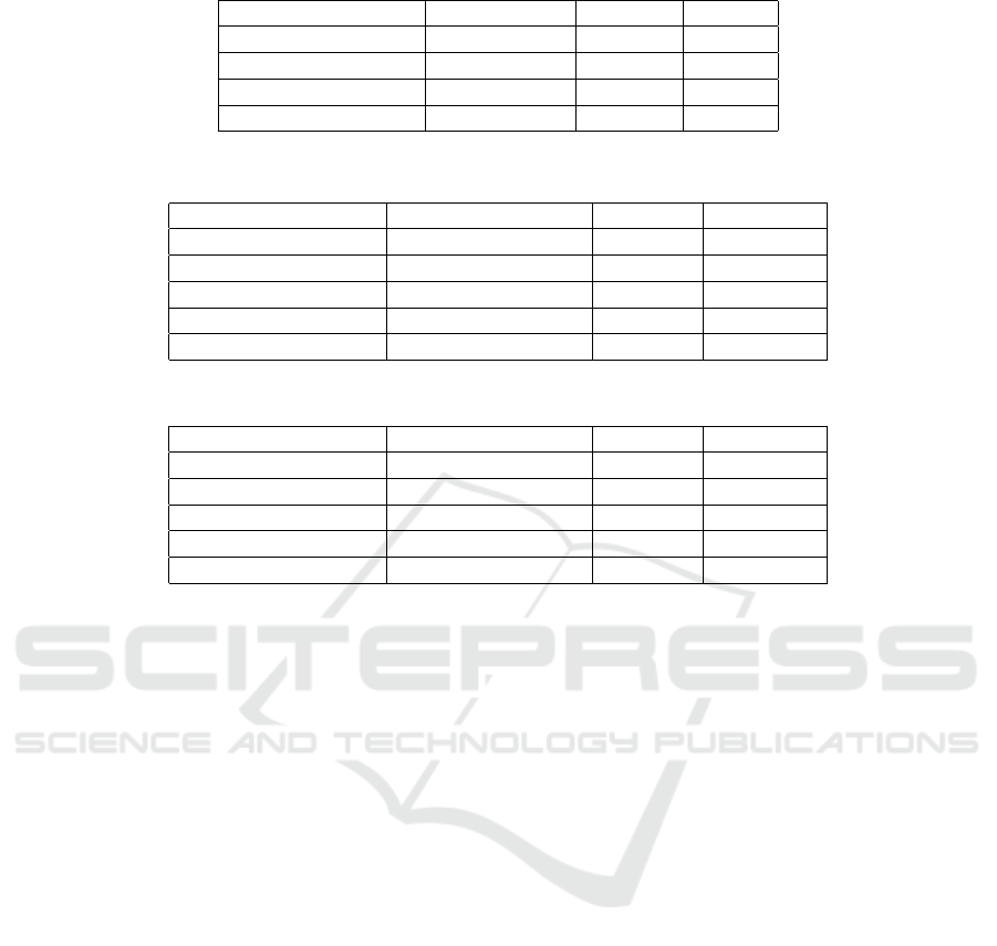
Table 3: CIFAR-10 algorithm progression summary.

Filter Dims Filters FCLs Acc

[[5, 5]] [32] [384, 10] 62.99%

[[3, 3]] [32] [384, 10] 62.55%

[[3, 3], [5, 5]] [32, 128] [384, 10] 72.03%

[[3, 3], [5, 5], [5, 5]] [32, 128, 256] [384, 10] 82.56%

Table 4: MNIST comparison with other methods.

Algorithm User Deﬁned Limits Accuracy Time (Hrs)

(Weka) Random Grid No 96.21% 400

RL No 99.56% 192

(Auto Weka) TPE No 81.97% 30

(Auto Weka) SMAC No 96.44% 30

PnP No 99.1% 4

Table 5: CIFAR-10 comparison with other methods.

Algorithm User Deﬁned Limits Accuracy Time (Hrs)

(Weka) Random Grid No 35.46% 400

RL No 92.68% 192

TPE Yes 82.53% 33

SMAC Yes 81.92% 33

PnP No 82.56% 7

ing exercise, but when it comes to ﬁnding an opti-

mal architecture for a speciﬁc application, it is the au-

thors’ argument that most practitioners cannot afford

the cost in time or expertise associated with that ap-

proach. In light of the cost associated with time and

expertise, the PnP approach is very favorable.

7 CONCLUSION

In conclusion, we can see that the PnP algorithm can

be applied to hyperparameter tuning of CNNs to ﬁnd

an optimal solution. It generates architectures that

give competitive results with signiﬁcantly less train-

ing time than other state of the art approaches.

There are a variety of ways that this work can be

extended in future work. For example, after running

PnP, a user may want to use the resulting architecture

as a starting point for a more localized random search.

Additionally, PnP results could be integrated into the

RL algorithm as a way to provide better quality inputs

to learn from. This could potentially reduce the train-

ing time currently required for the algorithm. For the

user that wants to do a lot of manual tweaking, PnP

can give a baseline to start from.

REFERENCES

Baker, B., Gupta, O., Naik, N., and Raskar, R. (2016). De-

signing neural network architectures using reinforce-

ment learning.

Bergstra, J., Bardenet, R., Bengio, Y., and Kgl, B. (2011).

Algorithms for hyper-parameter optimization. In Pro-

ceedings of the 24th International Conference on Neu-

ral Information Processing Systems, NIPS’11, pages

2546–2554. Curran Associates Inc.

Bergstra, J. and Bengio, Y. (2012). Random search for

hyper-parameter optimization. 13:281–305.

Chen, X.-Y., Peng, X.-Y., Peng, Y., and Li, J.-B. (2016).

The classiﬁcation of synthetic aperture radar image

target based on deep learning. Journal of Information

Hiding and Multimedia Signal Processing, 7:1345–

1353.

Domhan, T., Springenberg, J. T., and Hutter, F. (2015).

Speeding up automatic hyperparameter optimization

of deep neural networks by extrapolation of learn-

ing curves. In Proceedings of the 24th International

Conference on Artiﬁcial Intelligence, IJCAI’15, pages

3460–3468. AAAI Press.

Glorot, X. and Bengio, Y. (2010). Understanding the dif-

ﬁculty of training deep feedforward neural networks.

In Proceedings of the Thirteenth International Con-

ference on Artiﬁcial Intelligence and Statistics, pages

249–256.

He, K., Zhang, X., Ren, S., and Sun, J. (2015). Delving deep

into rectiﬁers: Surpassing human-level performance

on ImageNet classiﬁcation.

ICAART 2019 - 11th International Conference on Agents and Artiﬁcial Intelligence

394

Hinz, T., Navarro-Guerrero, N., Magg, S., and Wermter, S.

(2018). Speeding up the hyperparameter optimization

of deep convolutional neural networks.

Hutter, F., Hoos, H. H., and Leyton-Brown, K. (2011). Se-

quential model-based optimization for general algo-

rithm conﬁguration. In Proceedings of the 5th Inter-

national Conference on Learning and Intelligent Opti-

mization, LION’05, pages 507–523. Springer-Verlag.

Ioffe, S. and Szegedy, C. (2015). Batch normalization: Ac-

celerating deep network training by reducing inter-

nal covariate shift. arXiv:1502.03167 [cs]. arXiv:

1502.03167.

Kingma, D. P. and Ba, J. (2014). Adam: A method for

stochastic optimization.

Koch, P., Golovidov, O., Gardner, S., Wujek, B., Grifﬁn, J.,

and Xu, Y. (2018). Autotune: A derivative-free opti-

mization framework for hyperparameter tuning. pages

443–452.

Krizhevsky, A., Sutskever, I., and Hinton, G. E. (2017). Im-

ageNet classiﬁcation with deep convolutional neural

networks. 60(6):84–90.

LeCun, Y., Bengio, Y., and Hinton, G. (2015). Deep learn-

ing. Nature, 521(7553):436–444.

LeCun, Y., Bottou, L., Orr, G. B., and Mller, K.-R. (1998).

Efﬁcient BackProp. In Neural Networks: Tricks of

the Trade, This Book is an Outgrowth of a 1996 NIPS

Workshop, pages 9–50. Springer-Verlag.

Pu, L., Zhang, X., Wei, S., Fan, X., and Xiong, Z. (2016).

Target recognition of 3-d synthetic aperture radar im-

ages via deep belief network. In 2016 CIE Interna-

tional Conference on Radar (RADAR), pages 1–5.

Scherer, D., Mller, A., and Behnke, S. (2010). Evaluation

of Pooling Operations in Convolutional Architectures

for Object Recognition. In Diamantaras, K., Duch,

W., and Iliadis, L. S., editors, Artiﬁcial Neural Net-

works ICANN 2010, pages 92–101, Berlin, Heidel-

berg. Springer Berlin Heidelberg.

Schwegmann, C. P., Kleynhans, W., Salmon, B. P.,

Mdakane, L. W., and Meyer, R. G. V. (2016). Very

deep learning for ship discrimination in synthetic

aperture radar imagery. In 2016 IEEE Interna-

tional Geoscience and Remote Sensing Symposium

(IGARSS), pages 104–107.

Smith, L. N. (2017). Cyclical learning rates for training

neural networks.

Thornton, C., Hutter, F., Hoos, H. H., and Leyton-Brown,

K. (2012). Auto-WEKA: Combined selection and

hyperparameter optimization of classiﬁcation algo-

rithms.

Wang, S., Sun, J., Phillips, P., Zhao, G., and Zhang, Y.-

D. (2017). Polarimetric synthetic aperture radar im-

age segmentation by convolutional neural network us-

ing graphical processing units. DOI: 10.1007/s11554-

017-0717-0.

Plug and Play Deep Convolutional Neural Networks

395