Fast Non-minimal Solvers for Planar Motion Compatible Homographies

Marcus Valtonen

Ornhag

Centre for Mathematical Sciences, Lund University, Lund, Sweden

Keywords:

Planar Motion, Homography, Polynomial Solver, Trajectory Recovery, Visual Odometry.

Abstract:

This paper presents a novel polynomial constraint for homographies compatible with the general planar motion

model. In this setting, compatible homographies have ﬁve degrees of freedom—instead of the general case of

eight degrees of freedom—and, as a consequence, a minimal solver requires 2.5 point correspondences. The

existing minimal solver, however, is computationally expensive, and we propose using non-minimal solvers,

which signiﬁcantly reduces the execution time of obtaining a compatible homography, with accuracy and

robustness comparable to that of the minimal solver. The proposed solvers are compared with the minimal

solver and the traditional 4-point solver on synthetic and real data, and demonstrate good performance, in terms

of speed and accuracy. By decomposing the homographies obtained from the different methods, it is shown

that the proposed solvers have future potential to be incorporated in a complete Simultaneous Localization and

Mapping (SLAM) framework.

1 INTRODUCTION

Polynomial systems of equations naturally arise in the

ﬁeld of computer vision, as an instrument of encoding

geometric properties and other constraints one wishes

to impose on the desired output. To solve a gen-

eral system of polynomial equations, is, however, a

task requiring certain endeavour, in order to produce

a solver that is sufﬁciently fast and numerically stable.

In this paper we will investigate methods for Vi-

sual Odometry (VO), where the expected input is a

sequence of images from a camera mounted on a

mobile platform. The goal is to estimate the ego-

motion of the platform, in indoor environments or

other challenging scenes containing planar surfaces.

This is done by considering homography based meth-

ods, where we enforce the general planar motion

model. By imposing these constraints, thus lowering

the total degrees of freedom of the motion parameters,

it is possible to navigate robustly in scenes contain-

ing planar structures, which are problematic for VO

systems where a general structure of the scene is as-

sumed. It does, however, introduce a number of non-

trivial polynomial constraints, and a proper frame-

work for dealing with them must be employed.

The major contributions are:

i. To derive a new polynomial constraint for the gen-

eral planar motion model, and show that this, to-

gether with known constraints, are sufﬁcient con-

ditions for compatibility.

ii. To develop a series of non-minimal solvers to en-

force a weaker form of the general planar mo-

tion model, with a similar accuracy as the existing

minimal solver, at a greatly reduced speed.

iii. To demonstrate that pre-optimization on an early

stage in the intended VO pipeline, by enforcing

the general planar motion model on the homogra-

phies (but not a sequence of homographies), do

not necessarily give an increased performance.

2 RELATED WORK

Planar motion models with different complexity have

been considered to increase robustness of navigation

systems, by decreasing the total number of parameters

to be recovered. In (Ort

ın and Montiel, 2001) a mo-

bile platform with a single camera was considered,

where the optical axis was parallel to the ﬂoor. This

made it possible to parameterize the essential matrix

by imposing a planar motion model with two transla-

tional components and a single rotational component.

They propose a linear 3-point algorithm and a non-

linear 2-point algorithm; however, only the direction

of the translation can be recovered using their method.

Furthermore, the alignment of the optical axis with

the ﬂoor is not feasible for real-life applications. The

same geometrical setup was considered in (Chen and

Liu, 2006), but the algorithm was extended to stereo

vision.

Örnhag, M.

Fast Non-minimal Solvers for Planar Motion Compatible Homographies.

DOI: 10.5220/0007258600400051

In Proceedings of the 8th International Conference on Pattern Recognition Applications and Methods (ICPRAM 2019), pages 40-51

ISBN: 978-989-758-351-3

The fundamental matrix (or the essential matrix

in the calibrated case) have been successfully used in

many computer vision and robotics applications. De-

spite many promising navigation systems for general

scenes, such methods will not work well under pla-

nar motion, as it is known to be ill-conditioned (Hart-

ley and Zisserman, 2004; Torr et al., 1998). As

planar structures are common in man-made environ-

ments, researchers have considered alternative meth-

ods, many of which are based on inter-image homo-

graphies.

In (Hajjdiab and Lagani

ere, 2004) a planar mo-

tion model with one tilt parameter was considered,

and they proposed a method for estimating all mo-

tion parameters. By allowing an arbitrary tilt about

the ﬂoor normal Liang and Pears showed that the

eigenvalues of the homography matrix is related to

the rotation of the mobile platform, regardless of the

tilt (Liang and Pears, 2002). Their method, however,

did not estimate the tilt parameters.

The method proposed in (Wadenb

ack and Heyden,

2013; Wadenb

ack and Heyden, 2014) estimates the

full set of motion parameters for the general planar

motion model with ﬁve degrees of freedom by de-

coupling the overhead tilt using an iterative scheme.

From the same model assumption, but employing a

dense matching scheme, Zienkiewicz and Davison

devise a non-linear optimization scheme for the full

set of motion parameters (Zienkiewicz and Davison,

2015).

Without enforcing any model constraints, a gen-

eral homography has eight degrees of freedom; how-

ever, a homography compatible with the general

planar motion model only has ﬁve, as it is deter-

mined (up to scale) by the motion parameters. Due

to the automated process of extracting and match-

ing keypoints, homography solvers often employ

RANSAC, or similar frameworks, to reject outliers.

The number of iterations N required to select a set

of keypoints only containing inliers is dependent

on the size of the subset of keypoints n, the de-

sired probability p and inlier ratio w, by the well-

known relation N = log(1 − p)/log(1 − w

) (Fischler

and Bolles, 1981). One way of increasing the speed

of such an algorithm is to reduce the necessary num-

ber of iterations, i.e. to create a solver that only uses

the minimal number of point correspondences needed

for the application. Such a solver is known as a min-

imal solver. In line with this argument, it is natural

to consider a minimal homography solver compatible

with the planar motion model, which has been con-

structed in (Wadenb

ack et al., 2016). They parame-

terize the homography as a linear combination of the

basis elements of the null space of the corresponding

DLT system, with 2.5 DLT constraints, and construct

eleven quartic constraints on the homography matrix,

which results in a system of eleven quartic equations

in three variables. By generating the corresponding

ideal, a basis for the quotient space can be constructed

and the original problem solved by employing the ac-

tion matrix method (M

oller and Stetter, 1995). Their

derivation involves steps of manual selection of basis

monomials, which is a time-consuming task.

In (Kukelova et al., 2008) an automatic genera-

tor for polynomial systems was introduced, and sev-

eral improvements have been made in recent years

to increase the performance, see e.g. (Larsson and

Astr

om, 2016; Larsson et al., 2017a; Larsson et al.,

2017b; Larsson et al., 2018b). Such methods have

been successfully used in several computer vision ap-

plications, e.g. (Ventura et al., 2014; Zheng et al.,

2013).

Minimal solvers permit intrinsic constraints to be

enforced on the solutions, while minimizing the num-

ber of necessary iterations in a RANSAC framework;

however, there are cases when the minimal solvers are

sensitive to noise, see e.g. (Triggs, 1991), or when the

complexity of minimal solver is large, thus making it

very slow, see e.g. (Larsson et al., 2018a). Under such

circumstances constructing a non-minimal solver is a

viable option.

3 PLANAR MOTION

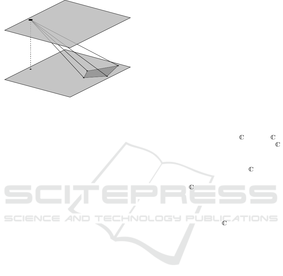
3.1 Problem Geometry

In this paper we consider a mobile platform with a sin-

gle camera directed towards the ﬂoor. The world co-

ordinate system is chosen such that the camera moves

in the plane z = 0. The scale is ﬁxed by assuming

the ground plane is positioned at z = 1, which is illus-

trated in Figure. 1.

We employ the parameterization used

in (Wadenb

ack and Heyden, 2013), where the

camera matrices for two consecutive poses A and B,

are given by

= R

ψθ

I | 0

0],

= R

ψθ

I | −t

t],

(1)

where R

ψθ

is a rotation θ about the y-axis followed

by a rotation ψ about the x-axis. As the mobile plat-

form rotates about the plane normal (or z-axis) the

angle φ varies, corresponding to R

. The translation

of the mobile platform is modelled by a translation

vector t

t = (t

, t

, 0)

. It follows that the inter-image

homography is given by

H ∼ R

ψθ

, (2)

Fast Non-minimal Solvers for Planar Motion Compatible Homographies

z = 1

plane normal

z = 0

Figure 1: The problem geometry considered in this paper.

The camera moves in the plane z = 0, and is tilted about the

y-axis an unknown angle θ, followed by a rotation about the

x-axis by an unknown angle ψ, The ground ﬂoor is posi-

tioned at z = 1.

where T

= I

I − t

is the translation matrix corre-

sponding to the translation t

t, and n

n = (0, 0, 1)

is a

ﬂoor normal. The homography matrix can be made

unique by imposing detH

H = 1, which will be assumed

throughout the paper.

3.2 Parameter Recovery

In (Wadenb

ack and Heyden, 2013) an algorithm for

recovering the full set of motion parameters for the

general planar motion model was suggested. Their

approach is to separate the overhead tilt R

ψθ

from the

nonconstant motion parameters. This can be achieved

using a coordinate-descent like optimization scheme,

where one of the tilt angles are ﬁxed and the other is

solved for. A more robust version by the same authors

was introduced in (Wadenb

ack and Heyden, 2014) by

using more than one homography, and incorporating

the assumption of a ﬁxed overhead tilt throughout the

entire trajectory of the mobile platform.

4 COMPATIBLE

HOMOGRAPHIES

The Direct Linear Transform (DLT) equations for

a pair of point correspondences x

x ↔

x, where

x = (x, y, 1)

and

x = (ˆx, ˆy, 1)

is given by





0 −x

ˆyx

0 − ˆxx

− ˆyx

ˆxx













= 0

0, (3)

where h

is the k:th row of the homography matrix H

It is only necessary to consider the ﬁrst two rows of

the DLT system matrix in (3), as the third is a lin-

ear combination of the others. We will use these

equations to parameterize the null space of the homo-

graphy matrix H

H in Section 6.

We will introduce some notation from algebraic

geometry in order to outline the method employed to

create the polynomial solvers we will consider in this

paper.

4.1 The Action Matrix Method

Consider a polynomial system of equations

x) = 0,

x) = 0 .

(4)

The set of all solutions to (4), is known as an afﬁne

variety, and denoted V

V ( f

,..., f

) ⊂ [x

x], where [x

is the set of polynomials in x

x with coefﬁcients in .

The ideal generated by f

,..., f

, is denoted

h f

,..., f

i =

(

∑

i=1

: h

,..., h

∈ [x

)

. (5)

Every ideal of [x

x] is ﬁnitely generated, thus, the

polynomial system of equations (4) is deﬁned by the

generated ideal.

Under the assumption that the system has ﬁnitely

many solutions, I = h f

,..., f

i is zero-dimensional

and the quotient space A = [x

x]/I is ﬁnite dimen-

sional (Cox et al., 2005). Let [ f ] = { f +h | h ∈ I} de-

note the coset and consider the operator T

: A −→ A,

deﬁned by T

([g]) = [ f g]. Since the quotient space A

is ﬁnite-dimensional this operation can be represented

by a matrix M

, which is known as the action matrix.

Furthermore, select a monomial basis for A, which we

denote B = {[x

]}

j∈J

. Typically, such a basis is ob-

tained by using an improved version of Buchberger’s

algorithm. When the action matrix M

= (m

i j

) acts

on the basis elements a linear combination of the

monomials forming the basis is obtained,

([x

]) = [ f x

] =

∑

i∈J

i j

] . (6)

Consequently, for x

x ∈ V (I),

f (x

x)x

∑

i∈J

i j

. (7)

The basis B may be represented by a vector b

b, and

since that (7) must hold for all basis elements, the

problem can be reduced to an eigenvalue problem,

given by

f (x

x)b

b(x

x) = M

b(x

x) . (8)

ICPRAM 2019 - 8th International Conference on Pattern Recognition Applications and Methods

By multiplying (4) by a set of monomials an

equivalent, but larger problem is obtained. The prob-

lem of ﬁnding a suitable monomial basis remains,

and there is no exact criterion for doing so; how-

ever, it is desirable to ﬁnd the minimal set of mono-

mials to make the problem solvable (or numerically

stable). The coefﬁcient matrix of the expanded ma-

trix is known as an elimination template, and numer-

ous attempts of optimizing these have been made,

see e.g. (Kukelova et al., 2008; Larsson and

Astr

om,

2016; Larsson et al., 2017b; Larsson et al., 2018b).

4.2 Necessary Conditions

In (Wadenb

ack et al., 2016) eleven quartic constraints

for planar motion compatible homographies were de-

rived, and used to create a minimal solver. These con-

straints were experimentally obtained by randomly

generating points on the manifold deﬁning the planar

motion compatible homographies. In order to be able

to work over a ﬁnite ﬁeld, the rotation matrices were

constructed using Pythagorean triplets, hence integer

versions of the problem were obtained. By doing so,

the coefﬁcients for the polynomials could be found.

With this approach, however, one cannot rule out the

existence of higher order polynomials, and thus, suf-

ﬁciency cannot be proven. We will approach this dif-

ferently in the next Section.

5 SUFFICIENT CONDITIONS

In this section, we will show that the eleven quartic

constraints discussed in Section 4.2 are necessary but

not sufﬁcient. Furthermore, we show that by adding

a sixth degree polynomial to the existing quartic con-

straints one may guarantee sufﬁciency. This is done

by a novel parameterization, which allows one to ef-

ﬁciently compute the relevant elimination ideal.

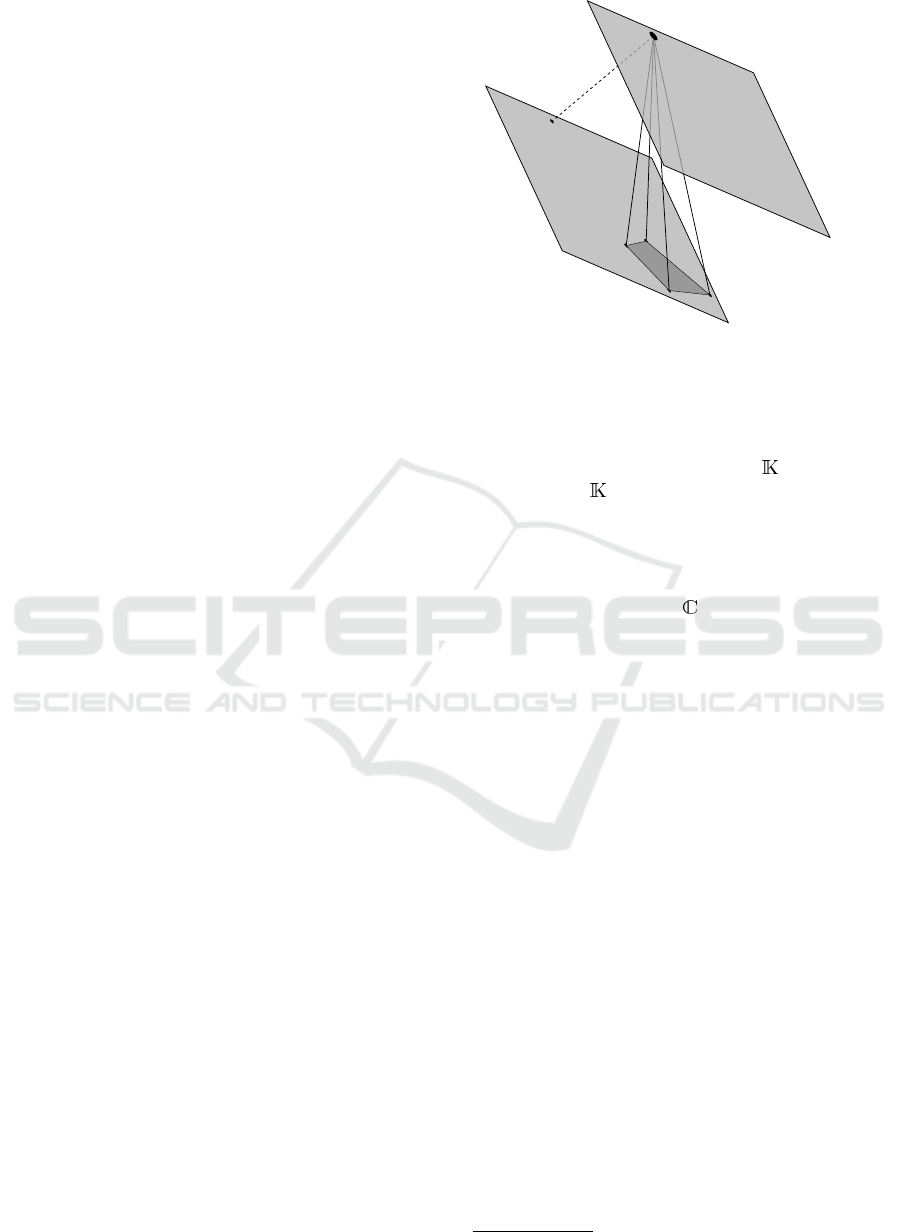
Instead of considering the original camera ma-

trices (1), choose the coordinate system such that

= [I

I |0

0], giving P

= [R

(φ)| − t

t]. This can be

thought of as travelling parallel to an unknown plane,

as is illustrated in Figure 2, hence the homography

can be parameterized as

H = R

(φ) + t

, (9)

where t

t = (t

, t

)

is a translation vector orthogo-

nal to the plane normal n

n = (n

, n

)

. The con-

straint of travelling parallel to the plane can be ex-

pressed as t

t · n

n = 0 and, to ﬁx the scale, one may as-

sume that kn

= 1.

Let q

q = (1, q

, q

) be a unit quaternion,

then n

n = (q

, q

) and the corresponding rota-

n = (n

, n

)

t · n = 0

knk

= 1

t = (t

, t

)

Figure 2: Revised problem geometry. The camera moves

parallel to an unknown plane deﬁned by a normal vector n

of unit length.

tion matrix R

R = R

R(q

q). Let the ideal generated by

λH

H −R

R(q

q) − t

= 0 and t

t · n

n = 0 be denoted I, then

we seek the elimination ideal I ∩ [H

H], for some

suitable ﬁeld . Over a ﬁnite ﬁeld, this can be

done using Macaulay2 (Grayson and Stillman, 2018).

This results in the eleven quartic constraints found

in (Wadenb

ack et al., 2016) and an additional sixth

degree polynomial

. The constraints were symboli-

cally veriﬁed to hold over as well.

6 NON-MINIMAL SOLVERS

In this section we consider different non-minimal

solvers as an alternative to the minimal solver pro-

posed in (Wadenb

ack et al., 2016). The main reason

we consider such solvers is due to the minimal solver

being computationally expensive. Also, there is no

advantage between a 2.5-point solver and a 3-point

solver, in terms of the number of iterations required to

select a subset of inliers with a certain probability—

this is a favourable trait, compared to the standard 4-

point DLT solver. Furthermore, we would like to ex-

plore different methods using the novel sixth degree

polynomial, derived in Section 5. Lastly, and most

importantly for practical applications, the condition

that the overhead tilt remains constant is not enforced

by using any of the described method, but is achieved

at a later step in the VO pipeline. Therefore, it is un-

certain if pre-optimizing the homographies will yield

a better end result.

In this paper we construct four different non-

minimal solvers

3pt(4+4) a 3-point solver enforcing two quartic

See the Appendix for implementation details.

Fast Non-minimal Solvers for Planar Motion Compatible Homographies

−3

−2.5

−2

−1.5

−1

−0.5

−3

−1

kH −

2.5pt

3pt(4+4)

3pt(4+6)

3.5pt(4)

3.5pt(6)

4pt

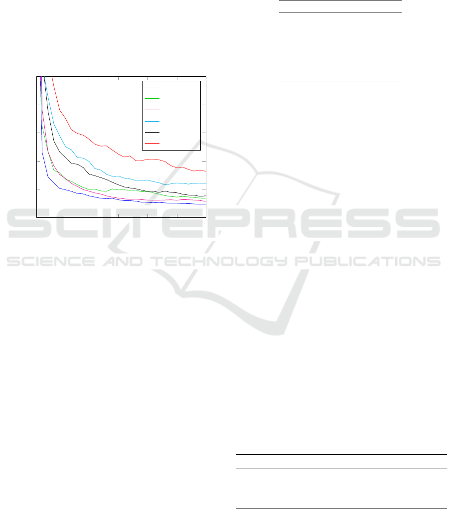
Figure 3: Distribution of homography error in the Frobenius norm for different noise levels σ

. The proposed non-minimal

solvers have a median error between the 2.5-point solver and DLT for all noise levels considered in the experiment.

constraints,

3pt(4+6) a 3-point solver enforcing one quartic

constraint and the sextic constraint,

3.5pt(4) a 3.5-point solver enforcing one quartic

constraint,

3.5pt(6) a 3.5-point solver enforcing the sextic

constraint.

These solvers were chosen because they enforce a

weaker version of the general planar motion model

in different ways. Furthermore, we will compare

with the minimal solver and the standard 4-point DLT

solver.

From the eleven quartic constraints the ﬁrst two

w.r.t. DEGLEX was chosen to construct the solvers;

however, this was only chosen for reproducibility, as

empirical tests showed that the size of the elimina-

tion template did not change by considering other

pairs. Similarly, when constructing the 3pt(4+6) and

3.5pt(4) solvers only the ﬁrst quartic constraint was

chosen.

6.1 Parameterizing the Null Space

The standard approach, which we will utilize, is to

parameterize the null space, and use the parameter-

ization to obtain the desired polynomial system of

equations. Using three DLT constraints (3) the homo-

graphy matrix H

H has a 3-dimensional null space,

hence can be parameterized as

H(z

z) = H

+ z

. (10)

Similarly, for the 3.5-point solvers, the null space is

two-dimensional, leaving a single variable. For such

systems, the action matrix method is replaced with a

simpler root ﬁnding algorithm, involving the compan-

ion matrix (Trefethen and Bau, 1997). In both cases

this allow the homography to be written as a func-

tion H

H = H

H(z

z), and inserted to any of the polyno-

mial constraints f

, yields an equation f

H(z

z)) = 0

in the variable z

z. For the 3-point solvers a system

of two equations are obtained, and the corresponding

ideal I = h f

, f

i can be studied. The number of basis

elements in the quotient space determines the number

of solutions (for non-degenerate conﬁgurations).

For the 3pt(4+4) solver the basis consists of 16

elements, hence the polynomial system of equations

has at most 16 solution. By using the automatic gen-

erator proposed by (Larsson et al., 2017a) an elimina-

tion template of size 20 × 36 was constructed. Due to

the increased complexity of the sextic constraint the

3pt(4+6) solver has in general 24 solutions, and the

corresponding elimination template is of size 31 × 55.

Furthermore, the coefﬁcients in the elimination tem-

plate are signiﬁcantly more complex.

7 EXPERIMENTS

7.1 Noise Sensitivity

In order to be comparable with the study of

noise sensitivity for the minimal solver proposed

in (Wadenb

ack et al., 2016), the same setup was used.

Homographies H

compatible with the general planar

motion model were generated together with randomly

generated keypoints x

with zero mean and unit vari-

ance. The image correspondences

∼ H

were

computed and normalized to unit variance. To sim-

ulate noise, a normal distributed term was added to

and

with standard deviation σ

. The homogra-

phies obtained from the solvers were normalized such

that det H

= 1, and the error measured in the Frobe-

nius norm of the difference between the ground truth

and the estimated homographies, see Figure 3. The

median sensitivity to noise of the proposed solvers

is between the corresponding values for the 2.5-point

solver and the 4-point (DLT) solver for all noise lev-

els, which indicates a trade-off between accuracy and

speed.

ICPRAM 2019 - 8th International Conference on Pattern Recognition Applications and Methods

Secondly, we generate a sequence of homogra-

phies compatible with the general planar motion

model, and use the method described in Section 3.2

to recover the motion parameters. For this example

the noise level was kept constant while increasing the

number of homographies used to estimate the motion

parameters. For σ

= 10

−2

the results are shown in

Figure 4. The results for the other motion parameters,

and different standard deviation σ

follow the same

trend, and can be found in the Appendix. Note, that

the mean error for the 3-point solvers are close to the

minimal solver after approximately 15 homographies

are used.

5 10 15 20 25 30

0.00

0.05

0.10

0.15

0.20

0.25

Number of homographies

Mean error ψ

2.5pt

3pt(4+4)

3pt(4+6)

3.5pt(4)

3.5pt(6)

4pt

Figure 4: Mean error for ψ (in degrees) for 100 iterations.

7.2 Speed Evaluation

The solvers were implemented in MATLAB, with

mex-compiled C++ routines. For a fair comparison,

the 2.5-point method and the 4-point (DLT) method

were also constructed this way. The 2.5-point method

was generated using the automatic solver by Lars-

son et al. (Larsson et al., 2017a), thus producing a

different elimination template than the one proposed

in (Wadenb

ack et al., 2016).

The execution time of the solvers was tested on

a standard laptop computer, and the measurements

include the complete process of estimating a homo-

graphy, i.e. staring from point correspondences, the

construction of the DLT system, extracting the null

space through SVD, and—except for the 4-point

solver—the parameter estimation for the basis ele-

ments of the null space, and construction of putative

homographies.

In Table 1 the timing comparison is shown, and

the speed-up between the minimal 2.5-point solver

and 3pt(4+4) solver is clear, however, in terms of

speed the traditional 4-point solver is faster. In a

complete RANSAC framework, however, the 3-point

solver and the 4-point solver is closer in terms of

speed, due to the 4-point solver requiring more iter-

ations to achieve the same probability of selecting a

subset containing only inliers.

Table 1: Mean execution time for 10,000 randomly gener-

ated problems.

Solver Exec. time (ms)

2.5pt 0.7960

3pt(4+4) 0.1334

3pt(4+6) 1.6161

3.5pt(4) 0.0344

3.5pt(6) 0.2919

4pt 0.0334

When enforcing the sixth degree polynomial in

the 3-point solver the number of solutions increase,

hence the corresponding elimination template. Fur-

thermore, the complexity of the coefﬁcients increase,

and this holds true in the case of the 3.5-point solvers

as well, which is why the execution time is faster

without the sextic constraint.

7.3 Synthetic Image Evaluation

A sequence of synthetic images were generated, com-

patible with the general planar motion model, by

cropping out images from a high-resolution image. In

order to simulate the overhead tilt the original image

was transformed prior to cropping it. An elliptic path

containing 49 images were generated, as well as the

corresponding ground truth.

The homographies were computed by extracting

and matching SURF features. In order to estimate the

trajectory, the homographies were decomposed us-

ing the method described in Section 3.2. The point

correspondences were normalized prior to estimat-

ing the homographies to increase numerical stability.

The extracted motion parameters were compared to

the ground truth. Due to the random nature of the

RANSAC, the recovered parameters were averaged

over 100 iterations. The results are shown in Table 2.

Table 2: Mean estimation error for the motion parameters

for the synthetic image test averaged over 100 iterations.

Angles are measured in degrees, and translation in pixels.

The best performance is in bold.

2.5pt 3pt(4+4) 3pt(4+6) 3.5pt(4) 3.5pt(6) 4pt

ψ 0.0035 0.0005 0.0029 0.0004 0.0006 0.0007

θ 0.0019 0.0006 0.0013 0.0005 0.0006 0.0007

φ 1.08 0.68 0.77 0.76 0.73 0.86

t 20.36 6.85 10.49 6.99 7.65 11.29

We observe that the minimal solver is no longer

producing the best results, and one may note the ad-

Fast Non-minimal Solvers for Planar Motion Compatible Homographies

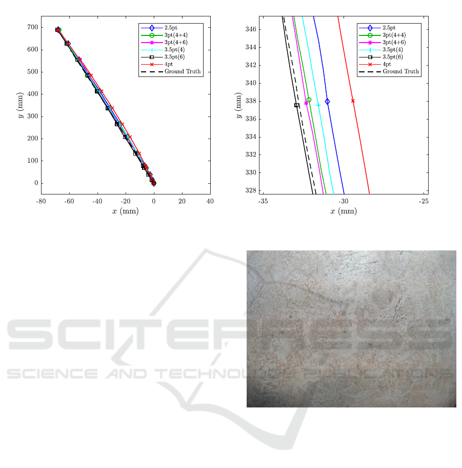
Figure 5: The sequence of the planar motion test set. The entire trajectory is shown to the left, and to the right a zoomed in

version showing the difference in estimates by using different solvers. The total sequence contains 320 images.

vantage of using non-minimal solvers. The exact rea-

son why this phenomenon arises when considering

synthetically generated sequences of images and not

synthetically generated sequences of homographies is

hard to pinpoint; however, we note the following dif-

ferences: (a) the matched points, which are the in-

put to the solvers do not follow a Gaussian distribu-

tion, and (b) when analyzing the numerical rank of the

elimination template it often has less than full rank,

which is not the case for the Gaussian distributed

noise. This holds true regardless of whether one nor-

malizes the image points or not. (c) the numerical

rank of the other elimination templates do not change

when going from synthetic homographies to synthetic

images.

7.4 Planar Motion Evaluation

The following experiments were conducted using a

mobile robot with omnidirectional wheels, of model

Fraunhofer IPA rob@work. A camera was mounted,

directed towards the ﬂoor, and the ground truth was

measured using a Nikon Metrology K600 optical

tracking system. The system has an absolute accuracy

of 100 µm. In Figure 6 example images from one of

the sequences are shown. In the ﬁrst test sequences

the robot travels along a straight line, while keeping

the orientation constant.

The same approach for computing the homogra-

phies in Section 7.3, after ﬁrst compensating for geo-

metric distortion. The results are shown in Figure 5,

and more test results are shown in the Appendix.

Note, that the minimal solver and the 4-point solver

are the ones to deviate the most from the ground truth

trajectory.

Figure 6: Example image from the planar motion sequence.

7.5 Evaluation on the KITTI Dataset

The KITTI Visual Odometry / SLAM bench-

mark (Geiger et al., 2012) is a well-known evalua-

tion dataset for SLAM frameworks, and contains sev-

eral sequences with planar or near planar motion. A

large portion of the images depict the roads, on which

the car travels, however, one must note that this is

only a coarse approximation to the general planar mo-

tion model, as all sequences contain non-planar struc-

tures to some extent, e.g. passing vehicles, pedestri-

ans, trafﬁc barriers and road signs. This, however, is

a good way of testing the robustness of the proposed

solvers, as future applications may not entirely ful-

ﬁll the general planar motion model. Furthermore, in

order to be able to consider the input images as de-

picting a (near) planar scene, a subset of the image is

cropped out before estimating the homographies, as is

illustrated in Figure 8.

ICPRAM 2019 - 8th International Conference on Pattern Recognition Applications and Methods

00 01 02 03 04 05 06 07 08 09 10

−2

−1

Sequence no.

Translation error (m)

2.5pt

3pt(4+4)

3pt(4+6)

3.5pt(4)

3.5pt(6)

4pt

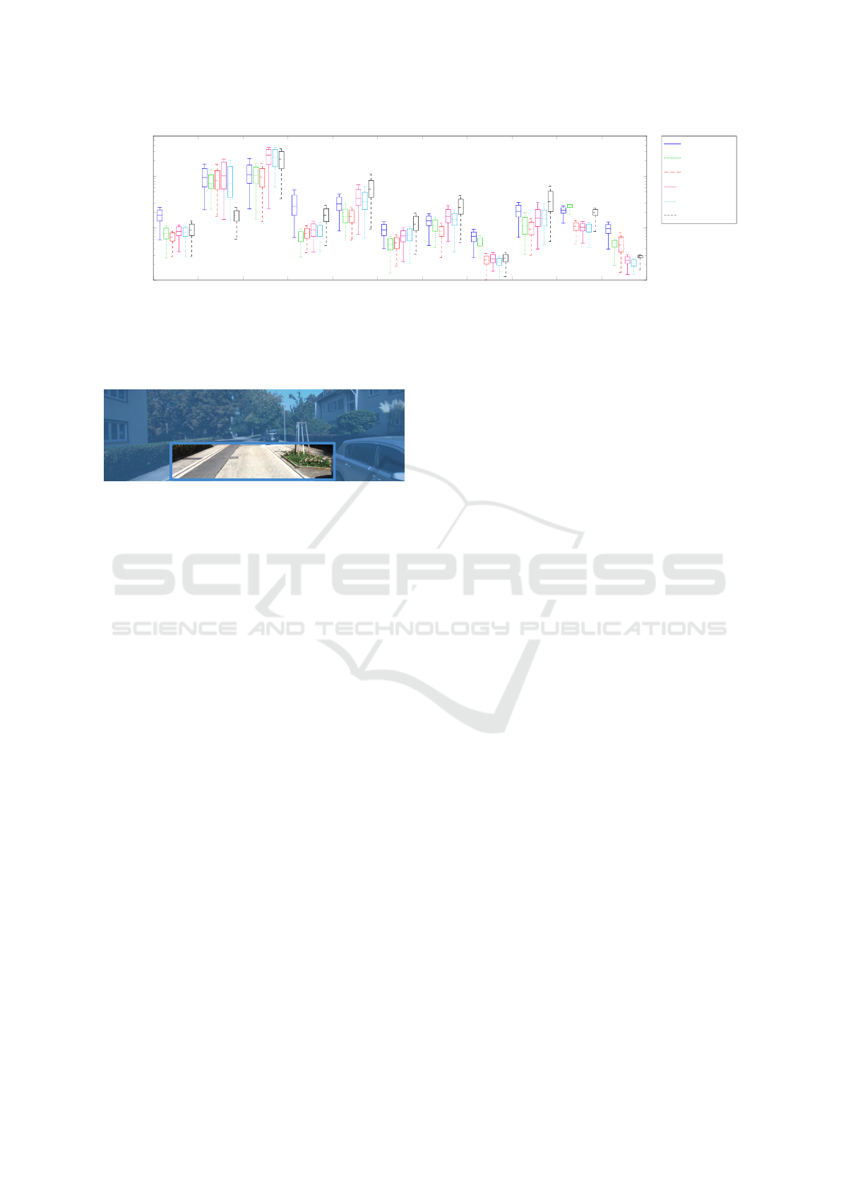
Figure 7: Mean translation error for the ﬁrst ten images of the ﬁrst camera of Sequence 00–10 of the KITTI dataset. These

are all image sequences containing ground truth. At least on of the proposed solvers have the lowest mean translation error in

all but one of the eleven cases. The mean translation error is computed over 500 iterations.

Figure 8: Image from the KITTI Visual Odometry / SLAM

benchmark, Sequence 03. The cropped area (contained

within the thick border) depict the image used to compute

the homographies. Image credit: KITTI dataset (Geiger

et al., 2012).

From the cropped images of the ﬁrst eleven se-

quences of the KITTI dataset, for which ground truth

data is available, the homographies were computed

using SURF features, as in the previous experiments.

The performance of the solvers was measured as the

mean error of the Euclidean distance between the

ground truth positions and estimated positions. The

results are averaged over 500 tests, and include the

ﬁrst ten images of each sequence. This number was

chosen to reduce the impact of error propagation,

while still having a noticeable effect of imposing the

general planar motion model. The differences of the

estimation is due to the matching algorithm as well as

the RANSAC framework for estimating the homogra-

phies. No non-linear reﬁnement of the homographies

were used. The results are shown in Figure 7.

The proposed solvers are robust, and produce a

good initial estimate for the trajectory, and at least one

of the proposed solvers has the lowest median trans-

lation error in all sequences, except Sequence 01.

This result may, to some extent, be unanticipated,

however, one must not forget that the conditions for

the general planar motion model is not fulﬁlled in the

KITTI dataset. The disadvantage of using the min-

imal 2.5-point solver, it seems, is that the model is

imposed exactly, whereas for the 4-point DLT solver,

the model is completely disregarded, and instead are

determined solely by the data. One possible an-

swer to the results we observe on the KITTI dataset,

which favours the proposed solvers, is that it enforces

a weaker form of the general planar motion model

(since only one or two of the deﬁning equations are

considered) and tunes to the data in cases where the

model assumptions are invalid.

8 CONCLUSIONS

In this paper a novel non-minimal polynomial con-

straint for homographies compatible with the general

planar motion model has been derived. A series of

non-minimal solvers have been proposed, which en-

forces one or two of the deﬁning constraints. They

have been demonstrated on synthetic and real data

to perform well, and two of them are reported to be

faster than the minimal solver.

In cases where the general planar motion model is

a coarse approximation of the actual scene it is likely

that the proposed solvers are more robust, compared

to both the minimal solver and the 4-point solver.

Hence, it has been demonstrated that pre-maturely en-

forcing the planar motion model, without incorporat-

ing the ﬁxed overhead tilt constraint, does not neces-

sarily yield a better end result.

By incorporating the proposed solver in a com-

plete SLAM system, it is likely that the total execution

time will decrease due to a lower number of iterations

needed by non-linear reﬁnement of poses and scene

points in a bundle adjustment framework.

ACKNOWLEDGMENTS

The author gratefully acknowledges M

arten

Wadenb

ack and Martin Karlsson for providing

the data for the planar motion compatible sequences.

Fast Non-minimal Solvers for Planar Motion Compatible Homographies

This work has been funded by the Swedish Research

Council through grant no. 2015-05639 ‘Visual

SLAM based on Planar Homographies’.

REFERENCES

Chen, T. and Liu, Y.-H. (2006). A robust approach for struc-

ture from planar motion by stereo image sequences.

Machine Vision and Applications (MVA), 17(3):197–

209.

Cox, D. A., Little, J., and O’Shea, D. (2005). Using Al-

gebraic Geometry. Graduate Texts in Mathematics.

Springer New York.

Fischler, M. and Bolles, R. (1981). Random sample consen-

sus: A paradigm for model ﬁtting with applications to

image analysis and automated cartography. Commu-

nications of the ACM, 24(6):381–395.

Geiger, A., Lenz, P., and Urtasun, R. (2012). Are we ready

for autonomous driving? The KITTI vision bench-

mark suite. Conference on Computer Vision and Pat-

tern Recognition (CVPR), pages 3354–3361.

Grayson, D. R. and Stillman, M. E. (2018). Macaulay2 –

a software system for research in algebraic geometry.

Available at http://www.math.uiuc.edu/Macaulay2/.

Hajjdiab, H. and Lagani

ere, R. (2004). Vision-based multi-

robot simultaneous localization and mapping. In

Canadian Conference on Computer and Robot Vision

(CRV), pages 155–162, London, ON, Canada.

Hartley, R. I. and Zisserman, A. (2004). Multiple View Ge-

ometry in Computer Vision. Cambridge University

Press, Cambridge, England, UK, second edition.

Kukelova, Z., Bujnak, M., and Pajdla, T. (2008). Automatic

generator of minimal problem solvers. European Con-

ference on Computer Vision (ECCV), pages 302–315.

Larsson, V. and

Astr

om, K. (2016). Uncovering symme-

tries in polynomial systems. European Conference on

Computer Vision (ECCV), pages 252–267.

Larsson, V.,

Astr

om, K., and Oskarsson, M. (2017a). Ef-

ﬁcient solvers for minimal problems by syzygy-based

reduction. Computer Vision and Pattern Recognition

(CVPR), pages 2383–2392.

Larsson, V.,

Astr

om, K., and Oskarsson, M. (2017b). Poly-

nomial solvers for saturated ideals. International

Conference on Computer Vision (ICCV), pages 2307–

2316.

Larsson, V., Kukelova, Z., and Zheng, Y. (2018a). Camera

pose estimation with unknown principal point. Com-

puter Vision and Pattern Recognition (CVPR), pages

2984–2992.

Larsson, V., Oskarsson, M.,

Astr

om, K., Wallis, A.,

Kukelova, Z., and Pajdla, T. (2018b). Beyond gr

obner

bases: Basis selection for minimal solvers. Computer

Vision and Pattern Recognition (CVPR), pages 3945–

3954.

Liang, B. and Pears, N. (2002). Visual navigation using

planar homographies. In International Conference

on Robotics and Automation (ICRA), pages 205–210,

Washington, DC, USA.

oller, H. M. and Stetter, H. J. (1995). Multivariate poly-

nomial equations with multiple zeros solved by matrix

eigenproblems. Numerische Mathematik, 70(3):311–

329.

Ort

ın, D. and Montiel, J. M. M. (2001). Indoor robot motion

based on monocular images. Robotica, 19(3):331–

342.

Torr, P. H. S., Zisserman, A., and Maybank, S. J. (1998).

Robust detection of degenerate conﬁgurations while

estimating the fundamental matrix. Computer Vision

and Image Understanding, 71(3):312 – 333.

Trefethen, L. and Bau, D. (1997). Numerical Linear Alge-

bra. SIAM.

Triggs, B. (1991). Camera pose and calibration from 4 or

5 known 3d point. International Conference on Com-

puter Vision (ICCV), pages 278–284.

Ventura, J., Arth, C., Reitmayr, G., and Schmalstie, D.

(2014). A minimal solution to the generalized pose-

and-scale problem. Computer Vision and Pattern

Recognition (CVPR), pages 422–429.

Wadenb

ack, M. and Heyden, A. (2013). Planar motion and

hand-eye calibration using inter-image homographies

from a planar scene. International Conference on

Computer Vision Theory and Applications (VISAPP),

pages 164–168.

Wadenb

ack, M. and Heyden, A. (2014). Ego-motion recov-

ery and robust tilt estimation for planar motion using

several homographies. International Conference on

Computer Vision Theory and Applications (VISAPP),

pages 635–639.

Wadenb

ack, M.,

Astr

om, K., and Heyden, A. (2016). Re-

covering planar motion from homographies obtained

using a 2.5-point solver for a polynomial system. In-

ternational Conference on Image Processing (ICIP),

pages 2966–2970.

Zheng, Y., Kuang, Y., Sugimoto, S.,

Astr

om, K., and Oku-

tomi, M. (2013). Revisiting the pnp problem: A fast,

general and optimal solution. International Confer-

ence on Computer Vision (ICCV), pages 2344–2351.

Zienkiewicz, J. and Davison, A. J. (2015). Extrinsics auto-

calibration for dense planar visual odometry. Journal

of Field Robotics (JFR), 32(5):803–825.

APPENDIX

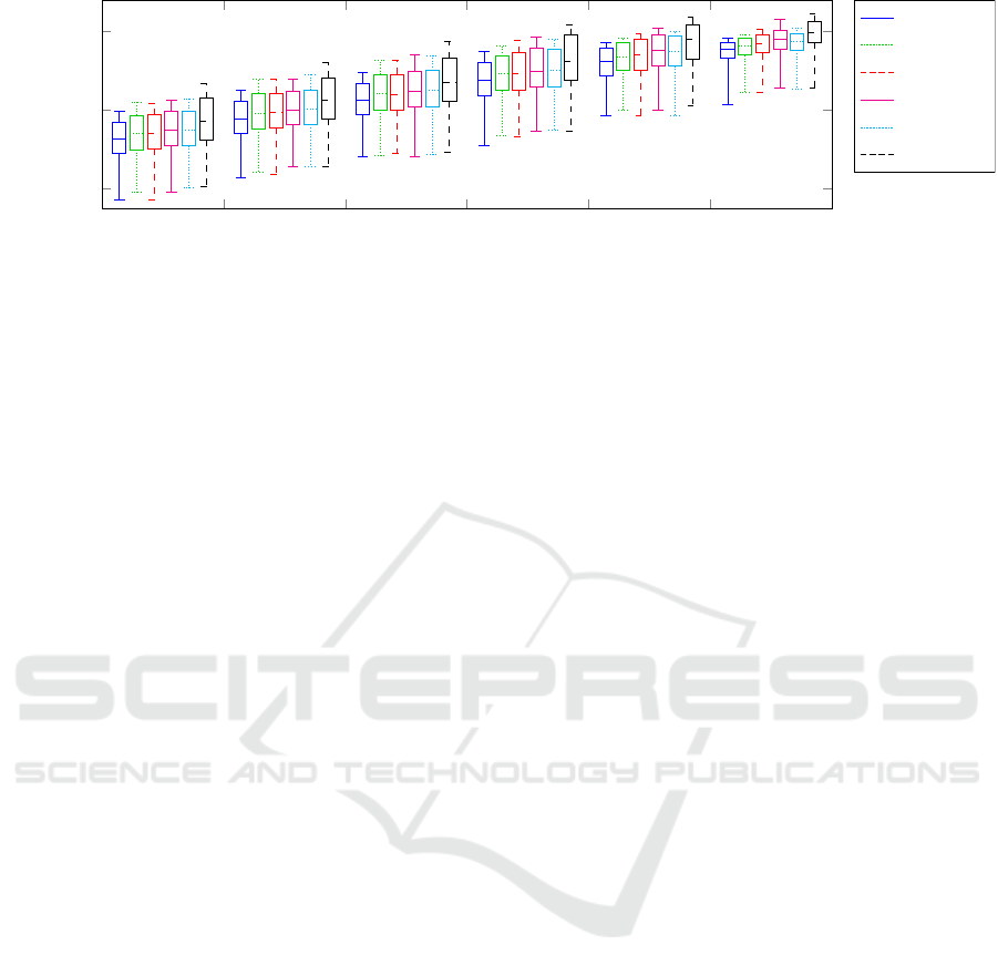
Synthetic Experiments

Re-projection Error

In (Wadenb

ack et al., 2016) the re-projection error for

the point correspondences not used in order to obtain

the estimated homographies were analysed, and we

reproduce it here together with the proposed solvers.

As seen in Figure 9, the trend is similar to what was

observed in the previous case (cf. Frobenius norm es-

timate, Figure 3) namely, the median re-projection er-

ICPRAM 2019 - 8th International Conference on Pattern Recognition Applications and Methods

−3

−2.5

−2

−1.5

−1

−0.5

−3

−1

Re-projection Error

2.5pt

3pt(4+4)

3pt(4+6)

3.5pt(4)

3.5pt(6)

4pt

Figure 9: Mean re-projection error for different noise levels σ

. Similar to Figure 3 the median value for the proposed solvers

is between the corresponding values for the 2.5-point solver and DLT; however, for higher noise levels, we note an advantage

for the non-minimal solvers and DLT compared to the minimal 2.5-point solver.

rors for the non-minimal solvers are between the cor-

responding values of the minimal 2.5-point solver and

the 4-point solver (DLT) for all noise levels. Note,

however, that for large noise levels, the 2.5-point

solver does not perform as well as the non-minimal

solvers or the traditional 4-point solver.

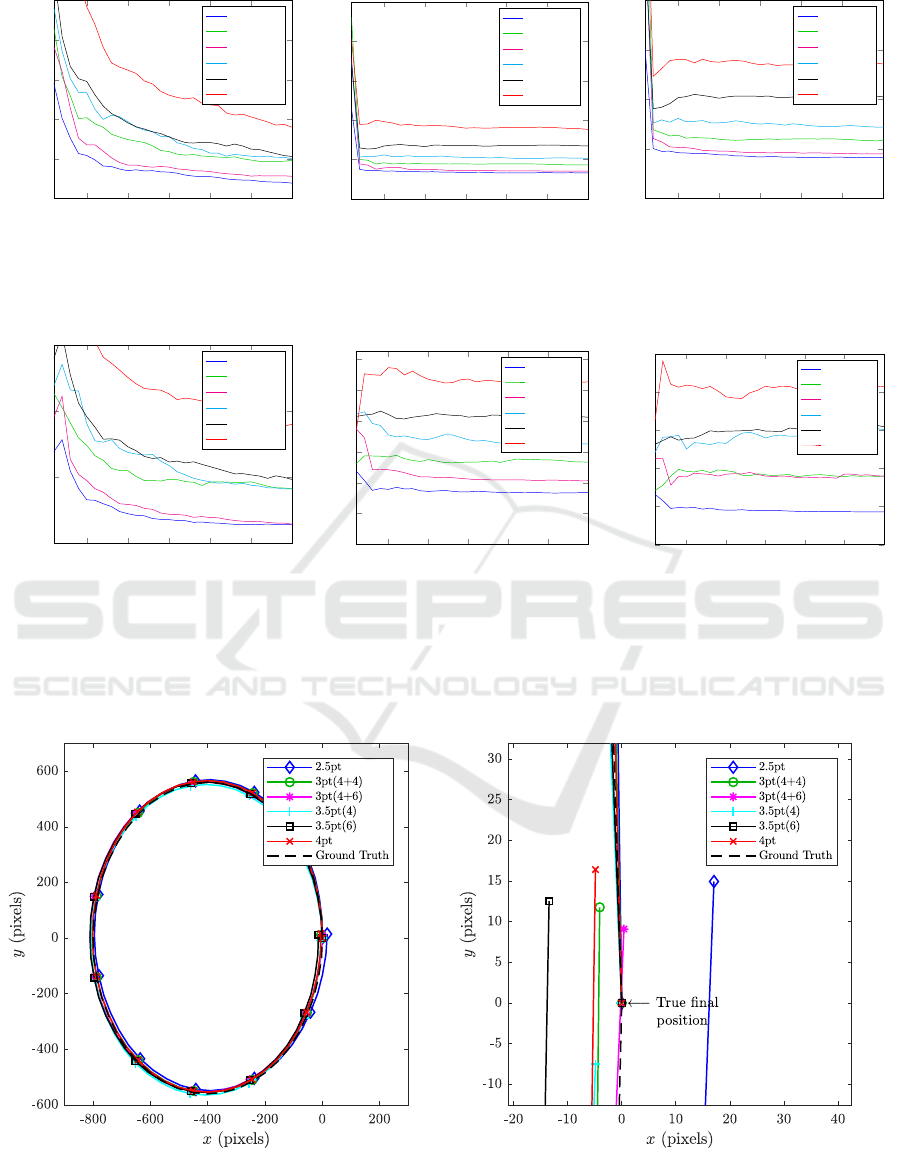
Motion Parameters

Additional plots for the second synthetic experiment,

regarding the estimation of the motion parameters, is

shown in Figure 11. The mean errors are for noise

level σ

= 10

−2

. In Figure 12 the same parameters,

but for σ

= 10

−1

are shown.

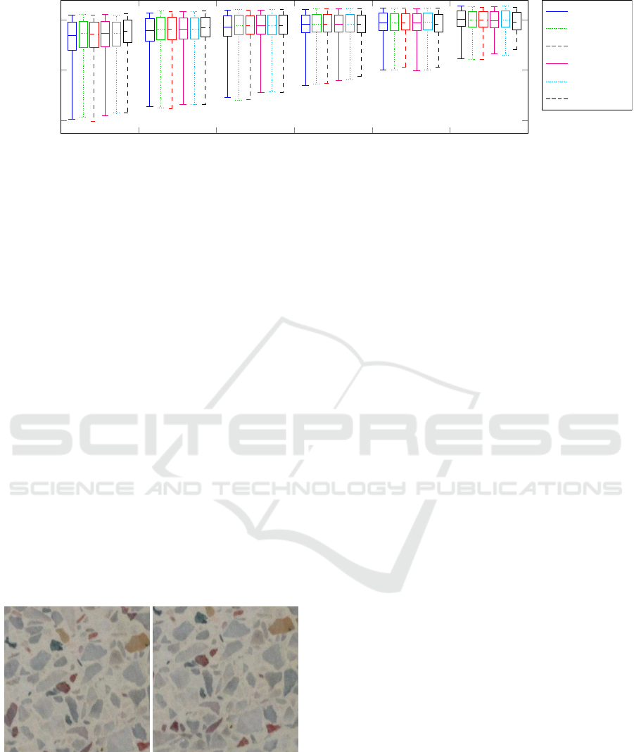
Synthetic Images

Example images that were used in the synthetic image

experiment is shown in Figure 10, and example output

for the reconstructed path is shown in Figure 13 for all

solvers. Neither the 4pt solver, nor the minimal solver

performs best in this case.

Figure 10: Two consecutive images from the synthetic

dataset.

Experiments on Real Data

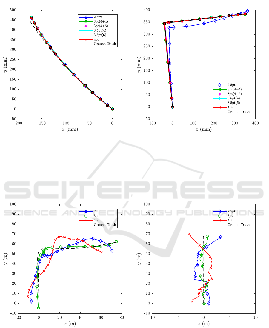
Planar Motion

We here show two more test cases conducted with the

omnidirectional robot rob@work, from Section 7.4.

In the ﬁrst test case the robot moves forward (in re-

lation to its own frame), while rotating, thus creating

a light turn. The sequence contains 344 images. In

the second test case the robot simulates a sequences

of parallel parking, by ﬁrst driving straight and then

making a sharp turn, while keeping the orientation

constant. This sequence contains 325 images. The

estimated paths are shown in Figure 14.

KITTI Dataset

To demonstrate some qualitative usage of the pro-

posed solvers, four longer subsequences of the KITTI

dataset were evaluated, see Figure 15. Only the

3pt(4 + 4) solver is shown in order to make the plots

legible. For sequences of this length it is customary

to use bundle adjustment, or some other non-linear

reﬁnement that minimize a physically meaningful er-

ror such as the geometric re-projection error or photo-

metric error. In order for such optimization schemes

to converge in a reasonable amount of time it is often

necessary to supply a good initial guess of the tra-

jectory. Due to the reduced computational complex-

ity, comparable to using the 4-point DLT solver, when

considered in a RANSAC framework, and the quali-

tative performance on the KITTI dataset, we ﬁnd the

proposed 3-point solver to be a suitable alternative to

be incorporated in a SLAM system.

Fast Non-minimal Solvers for Planar Motion Compatible Homographies

5 10 15 20 25 30

0.00

0.05

0.10

0.15

0.20

0.25

Number of homographies

Mean error θ

2.5pt

3pt(4+4)

3pt(4+6)

3.5pt(4)

3.5pt(6)

4pt

5 10 15 20 25 30

0.00

0.50

1.00

1.50

2.00

2.50

Number of homographies

Mean error φ

2.5pt

3pt(4+4)

3pt(4+6)

3.5pt(4)

3.5pt(6)

4pt

5 10 15 20 25 30

0.00

2.00

4.00

6.00

8.00

Number of homographies

Mean error t

2.5pt

3pt(4+4)

3pt(4+6)

3.5pt(4)

3.5pt(6)

4pt

Figure 11: Mean error for θ, φ (in degrees) and t

t for 100 iterations with σ

= 10

−2

5 10 15 20 25 30

0.00

1.00

2.00

3.00

Number of homographies

Mean error θ

2.5pt

3pt(4+4)

3pt(4+6)

3.5pt(4)

3.5pt(6)

4pt

5 10 15 20 25 30

0.00

2.00

4.00

6.00

8.00

10.00

12.00

Number of homographies

Mean error φ

2.5pt

3pt(4+4)

3pt(4+6)

3.5pt(4)

3.5pt(6)

4pt

5 10 15 20 25 30

0.00

20.00

40.00

60.00

80.00

100.00

Number of homographies

Mean error t

2.5pt

3pt(4+4)

3pt(4+6)

3.5pt(4)

3.5pt(6)

4pt

Figure 12: Mean error for θ, φ (in degrees) and t

t for 100 iterations with σ

= 10

−1

Figure 13: Example of reconstructed path for the synthetic image sequence for all solvers, and zoomed in at the ﬁnal position

(right image).

ICPRAM 2019 - 8th International Conference on Pattern Recognition Applications and Methods

(a) . (b) .

Figure 14: Estimated trajectories of the mobile robot used in the planar motion experiments for the “turn” experiment (left)

and the “parallel parking” experiment.

(a) Sequence 03 (200 images). (b) Sequence 04 (50 images).

Figure 15: Estimated trajectories of subsequences of Sequence 03 and 04 of the KITTI dataset. Procrustes analysis has been

carried out to align the estimated trajectories with the ground truth. Note that the aspect ratio differs between sequences, in

order to clearly visualize the differences between the estimated trajectories. No non-linear reﬁnement has been carried out in

any of the test cases. The 3-point solver used is the 3pt(4+4) solver.

Fast Non-minimal Solvers for Planar Motion Compatible Homographies