Eliminating Noise in the Matrix Proﬁle

Dieter De Paepe, Olivier Janssens and Soﬁe Van Hoecke

Ghent University – imec – IDLab, Department of Electronics and Information Systems, Ghent, Belgium

Keywords:

Matrix Proﬁle, Noise, Time Series, Anomaly Detection, Time Series Segmentation.

Abstract:

As companies are increasingly measuring their products and services, the amount of time series data is rising

and techniques to extract usable information are needed. One recently developed data mining technique for

time series is the Matrix Proﬁle. It consists of the smallest z-normalized Euclidean distance of each subse-

quence of a time series to all other subsequences of another series. It has been used for motif and discord

discovery, for segmentation and as building block for other techniques. One side effect of the z-normalization

used is that small ﬂuctuations on ﬂat signals are upscaled. This can lead to high and unintuitive distances for

very similar subsequences from noisy data. We determined an analytic method to estimate and remove the

effects of this noise, adding only a single, intuitive parameter to the calculation of the Matrix Proﬁle. This

paper explains our method and demonstrates it by performing discord discovery on the Numenta Anomaly

Benchmark and by segmenting the PAMAP2 activity dataset. We ﬁnd that our technique results in a more

intuitive Matrix Proﬁle and provides improved results in both usecases for series containing many ﬂat, noisy

subsequences. Since our technique is an extension of the Matrix Proﬁle, it can be applied to any of the various

tasks that could be solved by it, improving results where data contains ﬂat and noisy sequences.

1 INTRODUCTION

The amount of data available as time series is rapidly

increasing. This increase can be explained by the

lowering cost of sensors and storage, but also due to

the rising interest of companies to gain new insights

about their products or services. Areas of interest in-

clude pattern discovery (Papadimitriou and Faloutsos,

2005), anomaly detection (Wang et al., 2016) and user

load prediction (Vandewiele et al., 2017).

The Matrix Proﬁle is a recently developed data

mining technique for time series data that is calcu-

lated using two time series and a single intuitive pa-

rameter: the subsequence length m. It is a one-

dimensional series where each data point at a given

index represents the Euclidean distance between the

z-normalized (zero mean and unit variance) subse-

quence starting at that index in the ﬁrst time series

and the best matching (lowest distance) z-normalized

subsequence in the second time series. Both inputs

can be the same, meaning matches are searched for in

the same time series, in this case a trivial match buffer

prevents the subsequence matching itself or nearby

neighbours. The Matrix Proﬁle Index, which is calcu-

lated alongside the Matrix Proﬁle, contains the index

of the best match for each subsequence.

The Matrix Proﬁle can be used for motif discovery

(ﬁnding the best matching subsequence in a series),

discord discovery (ﬁnding the subsequence with the

largest distance to its nearest match) or as a building

block for other techniques such as segmentation, vi-

sualizing time series using Multidimensional Scaling

(MDS) (Yeh et al., 2017b) or ﬁnding gradually chang-

ing patterns in time series (Time Series Chains) (Zhu

et al., 2017). The Matrix Proﬁle has been applied to

various topics, including medical signals (Yeh et al.,

2016), query logs (Zhu et al., 2017) and music (Yeh

et al., 2017a).

The original STAMP algorithm is able to calcu-

late the Matrix Proﬁle in O(n

logn) time and O(n)

memory (Yeh et al., 2016). It uses the fact that the

z-normalized Euclidean distance between two vectors

can be calculated in constant time, given the dot prod-

uct of those two vectors, it calculates these dot prod-

ucts using the MASS algorithm (Mueen et al., 2015),

based on the Fast Fourier Transform. The later devel-

oped STOMP algorithm further improves this runtime

to O(n

) by reusing intermediate results.

A number of features/advantages of the Matrix

Proﬁle are:

• The only required parameter is the subsequence

length m, which has a clear meaning for users;

• The runtime to calculate the Matrix Proﬁle is in-

dependent of the chosen subsequence length m;

De Paepe, D., Janssens, O. and Van Hoecke, S.

Eliminating Noise in the Matrix Proﬁle.

DOI: 10.5220/0007314100830093

In Proceedings of the 8th International Conference on Pattern Recognition Applications and Methods (ICPRAM 2019), pages 83-93

ISBN: 978-989-758-351-3

Figure 1: Top: Three pairs of sequences with varying slopes

but exactly the same amount of noise. Bottom: The z-

normalized versions of the same sequences. We see how de-

pending on the slope, the Euclidean distance greatly varies

between the z-normalized sequences due to the ampliﬁca-

tion of the noise. The z-normalized Euclidean distances are

(from left to right): 7.61, 3.55 and 1.81.

• Using the STAMP algorithm, a very accurate

guess of the Matrix Proﬁle can be made in a frac-

tion of the time needed to calculate it;

• The algorithms to calculate the Matrix Proﬁle are

well suited for parallelization, as has been demon-

strated in a GPU implementation (Zhu et al.,

2016);

• The Matrix Proﬁle is not based on heuristics and

always provides an exact solution;

• No assumptions are made about the data, making

this technique domain agnostic.

Although z-normalization is important when com-

paring time series (Keogh and Kasetty, 2002), there is

one major downside: on a ﬂat signal, any ﬂuctuations

(noise) on the signal are enhanced, resulting in high

values in the Matrix Proﬁle. We demonstrate this in

Figure 1: we created 3 pairs of sequences, each con-

sisting of two lines having a speciﬁc slope. Each pair

has the exact same amount of noise added to both

lines. Despite the original sequences being equally

distant, the z-normalized sequences have a lower dis-

tance on the sloped lines. Since the Matrix Proﬁle

uses the z-normalized Euclidean distance, it is also

affected by this phenomenon.

Most use cases in literature relating to the Matrix

Proﬁle focus on processing time series where ﬂat se-

quences are rare or indicate periods of (uninterest-

ing) inactivity, these are not negatively affected by

this phenomenon. On the other hand, cases where ﬂat

patterns are relevant will suffer from the inﬂuence of

noise. As a preliminary example, observe Figure 4.

Here, we see a discord that is not picked up by the

Matrix Proﬁle due to the noise in the ﬂat areas of the

signal. We discuss this example in detail in Section 4.

Generally, the effects of ﬂat sequences might re-

sult in misleading or plain wrong insights. This is

problematic, since in many realistic cases a ﬂat se-

quence can occur and might simply indicates a steady

regime of the underlying process. Some cases and

their respective periods of ﬂat signals are: seismol-

ogy (periods of seismic inactivity), system monitor-

ing (similar metrics during a long running task - used

in Section 4) and movement monitoring (periods of

inactivity - used in Section 5). To improve the results

of the Matrix Proﬁle for these kinds of cases, we in-

vestigated and analytically estimated the inﬂuence of

noise on the Matrix Proﬁle, allowing us to negate it.

This paper is structured as follows: Section 2 lists

literature related to the Matrix Proﬁle. In Section 3 we

explain how to eliminate the effects of noise. Section

4 demonstrates the effect of our technique on anomaly

detection for a simple synthetic example and using

data from the Numenta Anomaly Benchmark (NAB).

In Section 5 we apply our technique to time series

segmentation on passive activities using the PAMAP2

dataset (Reiss and Stricker, 2012). We conclude our

ﬁndings in Section 6.

2 RELATED WORK

In this section we focus on related work speciﬁcally

about the Matrix Proﬁle.

The original Matrix Proﬁle paper (Yeh et al.,

2016) introduces the Matrix Proﬁle as a new method

for ﬁnding similarities in one-dimensional time series,

which can also serve for motif and discord discovery

as a side effect. The authors explain the STAMP and

STAMPI algorithms to calculate the Matrix Proﬁle in

batch and incremental steps respectively, based on the

MASS algorithm (Mueen et al., 2015). A later paper

(Yeh et al., 2017a) extends the Matrix Proﬁle to be

able to work with multi-dimensional data.

The STOMP algorithm, a faster version of

STAMP that reuses intermediary results in its calcu-

lation, is introduced in (Zhu et al., 2016). The same

paper describes how a GPU-based version of STOMP

(GPU-STOMP) was used to calculate the Matrix Pro-

ﬁle on a seismology dataset of 100 million datapoints

in only 12 days.

Yeh et al. describe how MDS, a data explo-

ration technique, does not work well when consid-

ering the subsequences in a time series (Yeh et al.,

2017b). Instead, it is useful to select representative

subsequences to use as input for MDS. When dealing

with discrete time series, the selection can be done

using the Minimum Description Length (MDL) and

Reduced Description Length (RDL), effectively se-

lecting subsequences that provide good compression.

The authors ﬁnd that the Euclidean distance is a good

proxy for RDL in real-valued time series, and can be

used to select the salient subsequences for display in

ICPRAM 2019 - 8th International Conference on Pattern Recognition Applications and Methods

MDS, meaning the Matrix Proﬁle can be used for this

task.

Sometimes the ﬁndings of the Matrix Proﬁle do

not coincide with the interests of the user, as they

might be interested in speciﬁc time frames, highly

variable patterns or in regions coinciding with activity

in another time series. Using a user-deﬁned Annota-

tion Vector, introduced in (Dau and Keogh, 2017), a

user can modify a Matrix Proﬁle, putting more focus

on the regions that he is interested in.

Time Series Chains are deﬁned in (Zhu et al.,

2017) as slowly changing, repeated patterns in time

series. To ﬁnd them, they deﬁne the left and right

Matrix Proﬁle, containing the distance to the best ear-

lier and later subsequences. They are calculated using

a modiﬁed version of STOMP that has the same com-

plexity.

The Matrix Proﬁle Index can be used to perform

time series segmentation: dividing a time series in in-

ternally consistent regimes (Gharghabi et al., 2017).

By examining the arcs deﬁned by the matches found

by the Matrix Proﬁle, they explain how a lower-than-

expected number of arcs at a speciﬁc timestamp gives

an indication of a change in the underlying system.

Their FLUSS algorithm and its online variant FLOSS

are found on average to outperform human segmen-

tation, based on experiments with 22 subjects and 12

data sets.

The Matrix Proﬁle has been used for various tech-

niques and applied to data from various domains.

However, data where ﬂat and noisy subsequences are

present has been mostly avoided in Matrix Proﬁle re-

lated literature, most likely due to the issue introduced

in Section 1. In fact, we suspect this issue will nega-

tively affect many applications of the Matrix Proﬁle,

severely limiting its applicability. To the best of our

knowledge, no technique has been published so far

to tackle the negative effects of ﬂat and noisy subse-

quences. In the following section, we will elaborate

on this issue and provide a solution for it.

3 ELIMINATING NOISE

In this section, we present our contribution: a way to

remove the effects of noise from the Matrix Proﬁle. In

Section 3.1, we ﬁrst estimate the effect of noise when

calculating the z-normalized Euclidean distance be-

tween identical sequences. Next, we present how to

use this estimate in the calculation of the Matrix Pro-

ﬁle in Section 3.2. Finally, we discuss the complexity

of the resulting algorithm in Section 3.3.

3.1 Estimating the Inﬂuence of Noise

In this section we will estimate the amount of noise

affecting the Matrix Proﬁle using statistical methods.

By taking this estimate into account while calculating

the Matrix Proﬁle, we will be able to greatly reduce

the inﬂuence of noise.

Assume we have a base sequence S

S ∈ R

and de-

rive two sequences X

X and Y

Y by adding Gaussian noise

and N

that was sampled from a normal distribu-

tion with variance σ

S = (s

, s

, . . . s

)

X = (s

+ n

, s

+ n

, . . . s

+ n

)

Y = (s

+ n

, s

+ n

, . . . s

+ n

)

Ideally, we would want the Euclidean distance be-

tween X

X and Y

Y to be zero, since they are both (noisy)

measurements of the exact same sequence S

S. Remem-

ber that the Matrix Proﬁle uses the Euclidean distance

of the z-normalized sequences.

D(X

X, Y

Y ) = EucDist(

Y )

= EucDist



X −µ

Y − µ



(

−

)

+ . . . + (

−

)

(1)

Here,

X denotes the z-normalized sequence, µ de-

notes the mean and σ the standard deviation.

We now determine the expected inﬂuence of the

noise. From here on, we consider the sequences as

random variables, and highlight this by referencing

them as X and Y .



D(X, Y )



= E



( ˆx

− ˆy

)

+ . . . + ( ˆx

− ˆy

)



= m · E



( ˆx − ˆy)



= m · E



x − µ

−

y − µ



(2)

Since X and Y are the sum of the same two uncor-

related variables, they both have the same variance.

= σ

+ σ

(3)

Furthermore, we can decompose µ

and µ

in the

original µ

and the inﬂuence of the noise. Here we

use n as the random variable sampled from the noise

distribution. Note that µ

can be seen as a constant.

Eliminating Noise in the Matrix Proﬁle

= µ

+ . . . + n

= µ

+ µ

∼ N





(4)

We can do the same for x and y, where s is an

unknown constant:

x = y = s + n

n ∼ N



0, σ



(5)

Using (3), (4) and (5) in (2), canceling out con-

stant terms and merging the distributions results in:



D(X, Y )



= m · E











− n

− µ

+ µ

+ σ











= m · E

(ν)

ν ∼ N



2 + 2m

+ σ



(6)

Finally, we apply the theorem E[X

] = var(X) +

E[X]



D(X, Y)



= (2m + 2) ·

+ σ

(7)

We now have an estimate of the distance between

two sequences that originate from the same sequence

but have been contaminated by Gaussian noise. Note

that in (7), σ

is the variance of the noise and σ

+σ

is the variance of the noisy sequence.

3.2 Algorithm for Noise Elimination

Implementing noise elimination is straightforward,

we subtract the squared estimate from the original

squared distance (e.g. as calculated by the MASS al-

gorithm). We do this before the element-wise mini-

mum is calculated and stored as value for the Matrix

Proﬁle, because this correction might inﬂuence which

subsequence gets chosen as the best match. Pseu-

docode is listed below.

Input: d # distance between subsequences X, Y

Input: m # length of each subsequence

Input: std_X # standard deviation of X

Input: std_Y # standard deviation of Y

Input: std_n # standard deviation of noise

d_corrected = sqrt(dˆ2 - (2 + 2m) * std_nˆ2 /

max(std_X, std_Y)ˆ2)

return d_corrected

Figure 2: Time measurements show the overhead of the

noise elimination, though the complexity remains O(n

Note that the maximum of the standard deviation

of both sequences is used. Given two fundamentally

different subsequences, this choice effectively mini-

mizes our estimate. We note that we tried other means

of combining the standard deviations such as mean

and minimum, but these produced similar results.

3.3 Complexity Analysis

The noise elimination is a constant operation if we

know the standard deviations, so complexity remains

O(n

logn) when using STAMP and O(n

) when us-

ing STOMP. This assumes the standard deviations for

all subsequences are precomputed, as is the case in

the STOMP and STAMP algorithms. A plot of the in-

ﬂuence of time series length versus runtime is shown

in Figure 2.

4 USE CASE: ANOMALY

DETECTION

One of the original applications for the Matrix Pro-

ﬁle was ﬁnding discords. Since discords are deﬁned

as the subsequences in a series that differ most from

any other subsequence, they can be interpreted as

anomalous subsequences. Since each Matrix Proﬁle

value represents the distance of each subsequence to

its nearest match, the top discord can be found triv-

ially given the Matrix Proﬁle: it is the subsequence

corresponding to the highest value. When interested

in the top-k discords, one can take the top-k values

of the Matrix Proﬁle where each value should be at

least m index positions away from all previous dis-

cord locations. Since overlapping subsequences are

very similar in shape, this prevents selecting the same

discord multiple times (Mueen et al., 2009).

In this section, we will use anomaly detection as

use case to demonstrate the inﬂuence of noise on the

Matrix Proﬁle. We ﬁrst focus on a small synthetic

dataset to provide details and insights, after which we

present results for real-world data from the Numenta

Anomaly Benchmark (Lavin and Ahmad, 2015).

ICPRAM 2019 - 8th International Conference on Pattern Recognition Applications and Methods

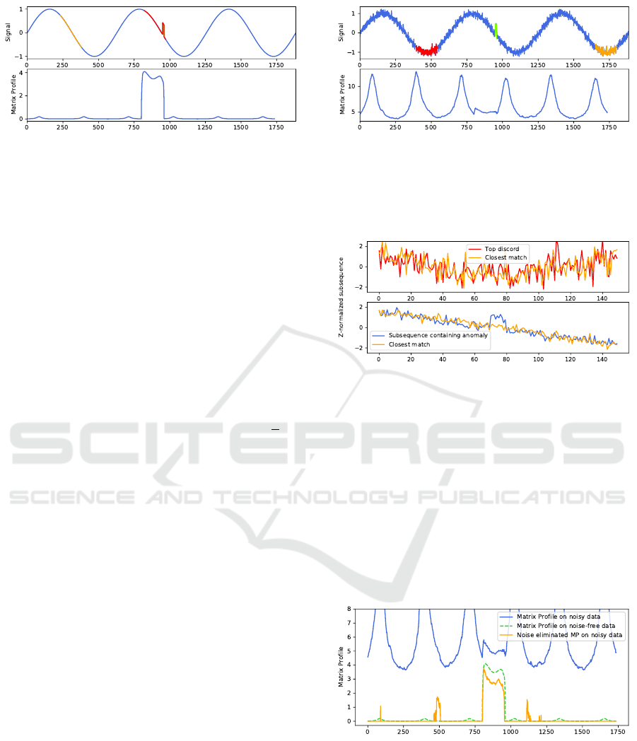
Figure 3: Top: Sinusoid signal, an anomaly of length 10

was added at index 950. The top discord (containing the

anomaly) and its closest match are highlighted in red and

orange. (The top discord subsequence starts at the highest

value of the Matrix Proﬁle.) Bottom: Corresponding Matrix

Proﬁle calculated with subsequence length m = 150. The

effect of the anomaly stands out as a series of high values.

4.1 Synthetic Data

We start from a synthetic dataset of 2000 samples of

a sinusoid in which we introduced an anomaly in one

of the downward slopes by increasing the value of 10

consecutive samples by 0.5. The dataset and corre-

sponding Matrix Proﬁle can be seen in Figure 3. Here,

we see how the Matrix Proﬁle clearly highlights the

subsequences containing the anomaly. For calculat-

ing the Matrix Proﬁle, we used a subsequence dis-

tance m of 150 and a trivial match buffer of

, as

recommended in (Yeh et al., 2016).

Next, we added Gaussian noise sampled from

N (0, 0.01) and recalculate the Matrix Proﬁle using

the same parameters. The resulting dataset and cor-

responding Matrix Proﬁle can be seen in Figure 4.

Although we see still the impact of the anomaly in

the Matrix Proﬁle as a deviation in the pattern, it

does not lead to a high value in the Matrix Proﬁle.

In a larger, more realistic dataset, this could mean

that the anomaly would go unnoticed. Instead, the

top-6 discords coincide with the ﬂat sections of the

sinusoid, where the noise has been upscaled due to

the z-normalization. This is visualized in Figure 5,

where we overlay the z-normalizations of the subse-

quences of the top discord and its best match with a

subsequence containing the data anomaly and its best

match. Since the Matrix Proﬁle consists of the Eu-

clidean distance between z-normalized subsequences,

more erratic z-normalized subsequences will typically

lead to higher distances.

After recalculating the Matrix Proﬁle using our

noise elimination technique from Section 3, the Ma-

trix Proﬁle again closely matches the Matrix Proﬁle

on the noise-free data, as can be seen in Figure 6.

Most subsequences now have a distance of zero, in-

dicating exact matches in the remainder of the se-

ries. The anomaly is again clearly visible and would

be marked as the top discord. Lastly, we see some

Figure 4: Top: Same signal as Figure 3, but with added

Gaussian noise. The anomaly is highlighted in green. The

top discord and its closest match are highlighted in red and

orange, they do not contain the data anomaly. Bottom: The

corresponding Matrix Proﬁle, the effect of the anomaly is

still visible but no longer stands out as a high value.

Figure 5: A close-up of the z-normalized subsequences

explains why the top discord has a higher Matrix Proﬁle

value than any subsequence containing the data anomaly.

The effect of the noise becomes larger due to the z-

normalization when the original subsequence is “ﬂatter”.

Top: z-normalized subsequence of the top discord and

its closest match (as marked in Figure 4). Bottom: z-

normalized subsequence that contains the data anomaly and

its closest match.

non-zero values not related to the anomaly, these are

caused by locally higher-than-expected noise values

in that part of the signal. It can be noted that these

values depend on the sampling of the noise and can in

fact be seen as subtle anomalies.

Figure 6: Plot of the Matrix Proﬁle for the noisy data (blue),

for noise-free data (dashed green) and for the noisy data, but

with the noise elimination applied (orange). We see that the

noise corrected Matrix Proﬁle closely matches the Matrix

Proﬁle of the noise-free data.

Let us brieﬂy further investigate how the proper-

ties of the noise affect the Matrix Proﬁle. Figure 7

displays our starting sinusoidal signal and anomaly,

to which Gaussian noise sampled from different dis-

Eliminating Noise in the Matrix Proﬁle

Figure 7: Top: Sinusoid signal with anomaly to which

Gaussian noise sampled from different distributions has

been added. Bottom: Corresponding Matrix Proﬁle cal-

culated with subsequence length m = 150 for each of the

noisy signals. We see how the Matrix Proﬁle becomes less

insightful as the amount of noise increases.

tributions was added. As expected, we see that as the

variation of the noise increases, the anomaly becomes

less apparent in the Matrix Proﬁle. The anomaly is no

longer visually obvious in the Matrix Proﬁle for noise

with variance of 0.25 or more. Somewhat surprising

is how quickly this effect becomes apparent: when the

noise has a variance of around 0.0004 (at this point the

signal-to-noise ratio is 1250 or 31 dB), the anomaly is

already occasionally overtaken as the top discord by

the ﬂat subsequences (depending on the sampling of

the noise). The noise cancellation technique becomes

unreliable once the variation is around 0.0625, and is

no longer useful for variations of 0.25 or higher. This

can be explained by the subtlety of our anomaly (an

increase by 0.5 for 10 time units), as high variance

noise can create similar artifacts. Note that these in-

sights are hard to generalize as a rule of thumb, as they

really depend on the properties of the time series, the

anomalies and the considered subsequence length.

Lastly, we discuss why some simple, seemingly

useful methods to tackle the effects of noise are not

generally usable.

• Changing the subsequence length m: as m be-

comes smaller, the effect of the anomaly on the

Matrix Proﬁle will indeed be bigger. However,

the effect of the noise also becomes bigger, result-

ing in a more eratic Matrix Proﬁle, still making it

hard to ﬁnd the actual anomaly. Without knowing

in advance what one is looking for, it is hard to

select a good value of m. This is demonstrated in

Figure 8 (top).

• Ignoring ﬂat sections: ignoring subsequences

whose variance is below a certain value would

result in removing the peaks in the Matrix Pro-

ﬁle. A ﬁrst problem is ﬁnding the correct cut-

off value, which is not trivial. Secondly, this ap-

proach would not be applicable in datasets where

ﬂat signals are the anomalies, or where matches

Figure 8: Approaches for negating the effects of noise that

do not work. Top: Matrix Proﬁle using different values for

the subsequence length m. Middle: Matrix Proﬁle while

ignoring subsequences with standard deviation below 0.2.

Bottom: Matrix Proﬁle after applying a Savitzky-Golay

smoothing and a Wiener frequency ﬁlter to the noisy data.

on ﬂat signals are useful, as is demonstrated in

the time series segmentation of Section 5. This

approach is demonstrated in Figure 8 (middle).

• Smoothing or ﬁltering: by preprocessing the noisy

signal, one could hope to remove the noise alto-

gether. Unfortunately, unless the speciﬁcs of the

noise are well known and the noise can be com-

pletely separated from the signal, there will al-

ways remain an amount of noise, resulting in the

same effects. This is demonstrated in Figure 8

(bottom).

4.2 Numenta Anomaly Benchmark

The Numenta Anomaly Benchmark (NAB) is a col-

lection of datasets, score metrics and supporting tools.

Most datasets are from real-world applications in dif-

ferent domains and have been annotated by hand

by multiple people and combined using a consen-

sus method. The benchmark is aimed at real-time

anomaly detectors, this is reﬂected in the scoring

method, where anomaly time windows are deﬁned and

detection in the start of the window is better rewarded.

We limited ourselves to the “realAWSCloud-

watch” collection, because this collection was the

only one that contained many ﬂat, noisy time series.

The collection consists of 17 datasets of real-world

data, measuring computer workload such as cpu uti-

lization, bytes written and request count. Each dataset

spans a time period of 4 to 16 days sampled at 5

minute intervals and contains 0 to 3 anomalies. One

dataset with 2 anomalies is visualized in Figure 9.

We did not use the score metric of the NAB, as

it requires labelling anomalies in a streaming fash-

ion, which would require optimizing a classiﬁcation

threshold for the Matrix Proﬁle. Instead, we relied

on the inherent ordering of normal to anomalous sub-

sequences that is captured in the Matrix Proﬁle: We

ICPRAM 2019 - 8th International Conference on Pattern Recognition Applications and Methods

Figure 9: Plot of the “rds cpu utilization cc0c53” dataset

from the Numenta Anomaly Benchmark, it contains 2

anomalies (dots) with associated anomaly windows (red).

calculated the Matrix Proﬁle over the time series and

counted how many guesses were needed to ﬁnd all

anomalies, with a limit of 10 wrong guesses. Note

that when calculating the Matrix Proﬁle, we only used

data from previous time steps to deﬁne normal behav-

ior, this is in line with the real-time anomaly detection

idea of the NAB and is needed to ensure we match

their deﬁnition of anomalous behavior.

We compare the performance of the Matrix Pro-

ﬁle with and without noise elimination. For each

dataset, we set the subsequence length equal to half

the anomaly time window (which is deﬁned by the

NAB as 10% of the data length, divided by the num-

ber of anomalies present). Furthermore, like in the

NAB, we use the ﬁrst 15% of the data as reference

data and do not report any anomalies in it. For the

noise elimination, we estimated the standard devia-

tion of the noise as the 5th percentile of the standard

deviations of all subsequences found in the reference

data. This value was similar to a manually estimated

value on a few test datasets and was selected as an

easy, automatically derivable value. Note that we did

not optimize the noise estimation value in any way.

Our results are listed in Table 1, where we see that

noise elimination has better results for 6 and worse re-

sults for 2 out of the 17 datasets. One of these worse

results can be explained because the reference data

contains a very noisy signal that later becomes more

stable, this causes an overestimation of the inﬂuence

of noise and results in exact matches being found for

the entire time series. More ﬁne grained control of

the noise parameter could likely correct this case. In

total, by using noise elimination, we found 28 out 30

anomalies, and made 56 wrong guesses in the pro-

cess. In comparison, the original approach found 24

anomalies and had 80 wrong guesses. These results

show that by using the noise elimination, anomalies

become generally more noticeable and false positives

are reduced in the Matrix Proﬁle, resulting in less time

lost by the experts who diagnose these reports.

5 USE CASE: SEGMENTING

TIME SERIES

Detecting changes in an underlying system based on

sensor measurements has a wide range of applica-

tions, such as identifying different speakers in an au-

dio recording, detecting system intrusion or data anal-

ysis in general. In this section we will perform time

series segmentation using the Corrected Arc Curve

(CAC), a technique based on the Matrix Proﬁle. The

CAC is calculated by the FLUSS algorithm or its on-

line variant, the FLOSS algorithm, all are introduced

in (Gharghabi et al., 2017).

The CAC is coined as a domain agnostic tech-

nique to perform semantic time series segmentation

at super-human performance on realistic datasets and

even on streaming data. Both FLUSS and FLOSS

work by analyzing the Matrix Proﬁle Index, which

contains the index of the closest match for each sub-

sequence in a time series. To calculate the CAC,

the number of arcs (each spanning between a subse-

quence and their respective best match) are counted

and divided by the expected amount of arcs if all

matches were determined by uniform sampling over

the entire time series. Assuming that homogeneous

segments will display similar behavior and heteroge-

neous segments will not, a low ratio is seen as evi-

dence of a change in the underlying system. The CAC

is a vector of the same length as the Matrix Proﬁle and

is typically restricted to values between 0 and 1, the

lower the value, the more evidence of a change in the

underlying system.

5.1 Evaluation on PAMAP2 Dataset

The PAMAP2 dataset (Reiss and Stricker, 2012) con-

tains sensor measurements of 9 subjects performing

a subset of 18 activities including: sitting, standing,

walking, ironing and so on. The measurements are

time series containing the output of a heart rate mon-

itor and 3 inertial measurement units (IMU) placed

on the chest, dominant wrist and dominant ankle of

each subject. Each IMU measured 3-D acceleration

data, 3-D gyroscope data and 3-D magnetometer data

at around 100 Hz. The time series are annotated with

the activity being performed by the subject or marked

as a transition region in between activities. The dura-

tion of each activity varies greatly, but most activities

last between 3 to 5 minutes.

The PAMAP2 dataset was used in (Yeh et al.,

2017a), where the authors used the Matrix Proﬁle to

classify the activities in passive and active activities.

Speciﬁcally, they note that the motif pairs in the pas-

sive actions are less similar and therefore less useful.

Eliminating Noise in the Matrix Proﬁle

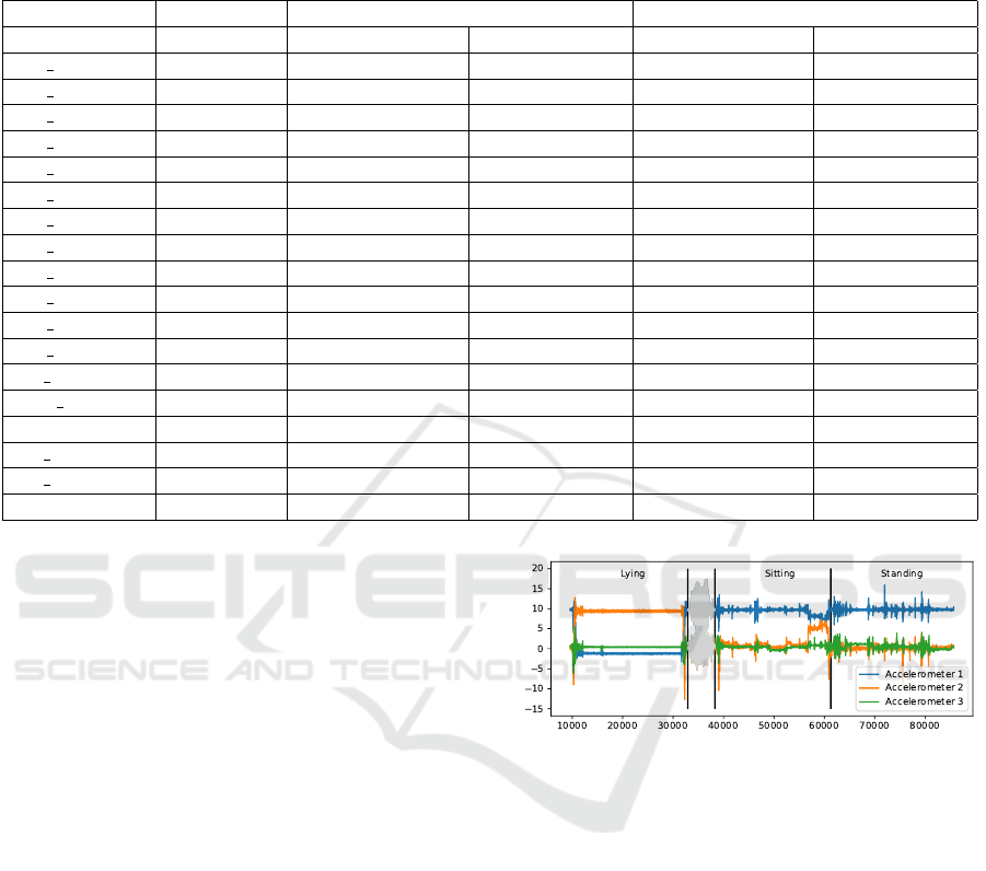
Table 1: Results of anomaly detection using the Matrix Proﬁle with and without noise elimination on the “realAWSCloud-

watch” collection of the Numenta Anomaly Benchmark. Each model kept guessing until all anomalies were found or until

10 wrong guesses occurred. Bold entries indicate a better performance of one approach over the other. We see that by using

noise elimination we can more easily ﬁnd the annotated anomalies in most cases.

Without Noise Elimination With Noise Elimination

Dataset #Anomalies Found Anomalies Wrong Guesses Found Anomalies Wrong Guesses

ec2 cpu...e8d 2 0 10 2 0

ec2 cpu...a38 2 2 6 2 0

ec2 cpu...533 2 2 1 2 10

ec2 cpu...1ca 1 0 10 1 9

ec2 cpu...cc2 1 1 0 1 0

ec2 cpu...0cd 1 1 1 1 0

ec2 cpu...85a 0 0 0 0 0

ec2 cpu...f93 3 1 10 1 10

ec2 disk...3de 1 1 3 1 3

ec2 disk...644 3 3 10 3 10

ec2 netw...a54 1 1 0 1 0

ec2 netw...ac7 2 2 3 2 3

elb reques... 2 2 10 2 0

grok asg... 3 3 3 3 3

ii...NetworkIn 2 2 0 2 5

rds cpu...c53 2 1 10 2 0

rds cpu...b3b 2 2 3 2 3

Sum 30 24 80 28 56

We argue that motifs in passive actions, consisting of

mainly ﬂat signals, can also help us ﬁnd structure in

the data if we can remove the inﬂuence of the noise.

We applied time series segmentation on the passive

activities present in the PAMAP2 dataset, focusing

on following activities: lying, sitting and standing.

We picked these activities since their measurements

display very few patterns in the data and they are con-

secutive activities for all subjects, meaning we did not

have to introduce time-jumps in the data.

We considered subjects 1 to 8 of the dataset (sub-

ject 9 has no recordings of the relevant activities) and

tested 2 cases: the transition from “lying” to “sit-

ting” and the transition from “sitting” to “standing”.

For each subject, we used the 3 accelerometer signals

from the IMU placed on the chest of the subject, any

missing data points were ﬁlled in using linear inter-

polation. We calculated the CAC with and without

noise elimination using a subsequence length of 1000

(10 seconds). The standard deviation of the noise was

estimated (without optimizing) by taking the 5th per-

centile of the standard deviations of all subsequences,

similar to our approach in Section 4.

An example of the signals can be seen in Figure

10. We emphasize it is not our goal to build the opti-

mal segmentation tool for this speciﬁc task, we simply

want to evaluate the effect of the noise elimination on

the CAC for sensor signals that contain ﬂat but noisy

Figure 10: Three chest accelerometers of subject 6 from

the PAMAP2 dataset. This extract contains 3 activities and

one transition period. No clear patterns are discernible and

many ﬂat and noisy subsequences are present.

subsequences.

There is one side effect of the noise cancellation

that needs attention before calculating the CAC. After

applying noise cancellation, many ﬂat subsequences

will have exact matches to other ﬂat subsequences.

However, since the Matrix Proﬁle Index can only

store a single match, the calculation order determines

which match actually gets stored. This causes an un-

wanted pattern in the Matrix Proﬁle indices, which

contradicts the assumption of the CAC that the struc-

ture of matches is related to similar segments. Note

that this effect is already present in the normal Matrix

Proﬁle, but typically has little to no inﬂuence because

multiple exact matches are extremely rare.

To solve this, we introduced reservoir sampling

(Vitter, 1985) to the construction of the Matrix Proﬁle

Index. Reservoir sampling allows uniform sampling

ICPRAM 2019 - 8th International Conference on Pattern Recognition Applications and Methods

without replacement from a stream without knowing

the size of the stream in advance. We implemented

reservoir sampling so that the Matrix Proﬁle Index no

longer stores the ﬁrst encountered best match, but a

uniformly sampled instance of all matches with the

lowest distance. This required us to store an addi-

tional vector of the same length as the Matrix Pro-

ﬁle, keeping track of the number of exact matches that

was encountered so far for each subsequence. Pseudo

code to update the Matrix Proﬁle and its indices is

listed below.

# Matrix Profile and Index being updated

Input: mp, mpi

# Distances (e.g. from STOMP iteration)

Input: dists

# Indices corresponding to dists

Input: indices

# Counts exact matches per subsequence

Input: match_counts

better_indices = dists < mp

eql_indices = dists == mp AND finite(dists)

mp(better_indices) = dists(better_indices)

mpi(better_indices) = indices(better_indices)

match_counts(better_indices) = 1

match_counts(eql_indices) += 1

for i in eql_indices:

if rand() < 1 / match_counts(i):

mpi(i) = indices(i)

return (mp, mpi)

For both test cases (lying-sitting and sitting-

standing), we calculated the CAC using the reser-

voir sampled Matrix Proﬁle indices with and without

noise elimination for each individual sensor. From the

CAC, we derived a single activity-transition point by

taking the location where the CAC is minimal. We

considered 4 segmentations: one for each CAC of the

3 sensor channels and one obtained by combining (av-

eraging) these individual CACs.

For scoring, we wish to reward splits on or near

the transition periods as annotated in the data sets.

Note that some transitions are instantaneous, while

others consist of a transient period, as can be seen in

Figure 10. We added a buffer margin of subsequence

size m to the transitions, so each transition period is at

least 2m wide. As score, we took the distance between

the estimated transition location and the buffered tran-

sition period, normalized by the length of the series

(containing both activities and the transition period).

Pseudo code for this scoring function is listed below,

a score will range from 0 to 100, where lower is better.

Table 2: Score for the segmentation of the transition from

“lying” to “sitting” using the 3 chest accelerometers from

the PAMAP2 dataset for subjects 1 through 8, with and

without noise elimination applied. Segmentation is per-

formed using the CAC from a single sensor (C1, C2 and

C3) and using the combined CAC. We see similar or better

performance when applying noise elimination for all sub-

jects except subject 1.

Without NE With NE

Subj. C1 C2 C3 Comb. C1 C2 C3 Comb.

1 5.9 31.3 31.9 31.7 41.3 31.8 41.8 36.7

2 32.9 1.4 1.4 1.4 28.8 1.4 1.7 1.4

3 35.9 2.8 31.1 33.8 2.4 2.3 2.3 2.3

4 0.0 2.8 5.9 0.0 0.0 1.5 6.6 0.8

5 1.1 7.6 5.1 3.9 1.6 1.7 4.9 1.6

6 2.5 1.9 2.3 2.3 2.4 1.9 2.0 2.4

7 0.1 1.8 11.1 2.0 2.1 1.8 1.9 1.9

8 0.0 1.4 5.5 1.7 0.0 1.4 1.4 1.4

Avg. 9.32 9.61 7.71 6.07

Table 3: Score for the segmentation of the transition from

“sitting” to “standing” using the 3 chest accelerometers

from the PAMAP2 dataset for subjects 1 through 8, with

and without noise elimination applied. Segmentation is per-

formed using the CAC from a single sensor (C1, C2 and

C3) and using the combined CAC. Overall, we see similar

or better performance when applying noise elimination, ex-

cept for the segmentation using the ﬁrst channel for subject

1, 3 and 8.

Without NE With NE

Subj. C1 C2 C3 Comb. C1 C2 C3 Comb.

1 32.5 0.0 3.6 2.2 38.7 0.0 3.7 2.2

2 36.5 37.2 36.4 37.0 7.1 30.0 32.7 29.2

3 10.0 30.2 43.1 30.2 43.2 14.0 43.7 30.2

4 7.8 1.9 1.1 1.2 0.7 2.0 1.3 1.3

5 13.1 0.0 28.5 10.6 13.3 1.0 1.2 1.0

6 36.1 36.6 26.9 36.6 23.3 3.4 26.5 3.2

7 43.1 38.0 16.5 16.5 43.4 1.6 0.0 1.6

8 2.3 1.0 24.8 1.0 21.1 0.0 16.5 1.0

Avg. 21.12 16.9 15.35 10.3

Input: est_split # Algorithmic estimate

Input: split_start, split_end # Ground truth

Input: n # Length of the time series

Input: b # Buffer for transition

if est_split < split_start - b:

return ((split_start - b) - est_split)/n

elif est_split > split_end + b:

return (est_split - (split_end + b))/n

else:

return 0.

The results for segmentation on the transition

from “lying” to “sitting” are listed in Table 2. We see

that segmentation using the individual sensors as well

as the combined approach provides similar or better

results when using noise elimination for all subjects

except for subject 1. The average score for the indi-

vidual sensors improves from 9.32 to 7.71, a modest

improvement corresponding to a gain of about 8 sec-

onds. The segmentation based on all 3 sensor series

improves from 9.61 to 6.07, a gain of about 18.5 sec-

onds. The results for subject 1 can be attributed to

Eliminating Noise in the Matrix Proﬁle

changes of the subjects body position near the start

of the “lying” activity. This results in a lower-than-

expected amount of matches near the start, causing

the transition to be guessed too early. Note that both

techniques have trouble with subject 1.

Table 3 lists the results for the transition from

“sitting” to “standing”. Again, we see similar or

improved results when applying noise elimination,

except for 3 subjects using the ﬁrst sensor series.

Though results are worse compared to Table 2, the

gain by using noise elimination is more signiﬁcant.

When using a single sensor, results on average im-

prove from 21.12 to 15.35, corresponding to a gain of

about 27 seconds. If segmentation uses all 3 sensors,

results change from 16.9 to 10.3 on average, a gain of

around 31 seconds.

6 CONCLUSION

In this paper we discussed techniques and applica-

tions related to the Matrix Proﬁle. Our contribution

consists of a method to remove the effects of Gaussian

noise on the time series when calculating the Matrix

Proﬁle, without affecting the complexity of the un-

derlying algorithm. This method is based on a sta-

tistical analysis of the effects of z-normalized noisy

sequences on the Euclidean distance. The only re-

quirement for this technique is to know the variance

of the noise, which is an intuitive measure and can

be easily estimated by manually extracting a ﬂat but

noisy segment from the time series.

As the Matrix Proﬁle is widely usable for a va-

riety of problems and across various domains, so

is our technique. In this paper, we showed gains

for anomaly detection and time series segmentation.

Both cases were evaluated on public datasets contain-

ing real-word data and showed an improvement of

the results. On the Numenta Anomaly Benchmark,

we were able to retrieve more anomalies with less

guesses, saving an operator valuable time. On the

PAMAP2 dataset, we were able to more accurately

predict transitions between passive activities. We fo-

cused on datasets containing ﬂat and noisy segments,

a subject that was not yet tackled in other Matrix Pro-

ﬁle related literature.

Further work can be done on using a dynamic

value for the noise estimation, for series where noise

does not originate from measurement, but rather from

the underlying process.

ACKNOWLEDGEMENTS

This work has been carried out in the framework

of the Z-BRE4K project, which received funding

from the European Union’s Horizon 2020 research

and innovation programme under grant agreement no.

768869.

REFERENCES

Dau, H. A. and Keogh, E. (2017). Matrix Proﬁle V: A

Generic Technique to Incorporate Domain Knowledge

into Motif Discovery. In Proceedings of the 23rd

ACM SIGKDD International Conference on Knowl-

edge Discovery and Data Mining - KDD ’17, pages

125–134, New York, New York, USA. ACM Press.

Gharghabi, S., Ding, Y., Yeh, C.-C. M., Kamgar, K.,

Ulanova, L., and Keogh, E. (2017). Matrix Pro-

ﬁle VIII: Domain Agnostic Online Semantic Seg-

mentation at Superhuman Performance Levels. In

2017 IEEE International Conference on Data Mining

(ICDM), pages 117–126. IEEE.

Keogh, E. and Kasetty, S. (2002). On the need for time

series data mining benchmarks. Proceedings of the

eighth ACM SIGKDD international conference on

Knowledge discovery and data mining - KDD ’02,

page 102.

Lavin, A. and Ahmad, S. (2015). Evaluating Real-

Time Anomaly Detection Algorithms – The Numenta

Anomaly Benchmark. In 2015 IEEE 14th Interna-

tional Conference on Machine Learning and Applica-

tions (ICMLA), pages 38–44. IEEE.

Mueen, A., Keogh, E., Zhu, Q., Cash, S., and Westover, B.

(2009). Exact Discovery of Time Series Motifs. In

Proceedings of the 2009 SIAM International Confer-

ence on Data Mining.

Mueen, A., Viswanathan, K., Gupta, C., and Keogh,

E. (2015). The fastest similarity search al-

gorithm for time series subsequences under eu-

clidean distance. url: www. cs. unm. edu/˜

mueen/FastestSimilaritySearch. html (accessed 24

May, 2016).

Papadimitriou, S. and Faloutsos, C. (2005). Streaming Pat-

tern Discovery in Multiple Time-Series. International

Conference on Very Large Data Bases (VLDB), pages

697–708.

Reiss, A. and Stricker, D. (2012). Introducing a new bench-

marked dataset for activity monitoring. In Proceed-

ings - International Symposium on Wearable Comput-

ers, ISWC, pages 108–109.

Vandewiele, G., Colpaert, P., Janssens, O., Van Herwe-

gen, J., Verborgh, R., Mannens, E., Ongenae, F., and

De Turck, F. (2017). Predicting train occupancies

based on query logs and external data sources. In Pro-

ceedings of the 7th International Workshop on Loca-

tion and the Web.

ICPRAM 2019 - 8th International Conference on Pattern Recognition Applications and Methods

Vitter, J. S. (1985). Random sampling with a reser-

voir. ACM Transactions on Mathematical Software

(TOMS), 11(1):37–57.

Wang, X., Lin, J., Patel, N., and Braun, M. (2016). A

Self-Learning and Online Algorithm for Time Series

Anomaly Detection, with Application in CPU Manu-

facturing. In Proceedings of the 25th ACM Interna-

tional on Conference on Information and Knowledge

Management - CIKM ’16, pages 1823–1832, New

York, New York, USA. ACM Press.

Yeh, C.-C. M., Kavantzas, N., and Keogh, E. (2017a). Ma-

trix Proﬁle VI: Meaningful Multidimensional Motif

Discovery. In 2017 IEEE International Conference

on Data Mining (ICDM), pages 565–574. IEEE.

Yeh, C. C. M., Van Herle, H., and Keogh, E. (2017b). Ma-

trix proﬁle III: The matrix proﬁle allows visualization

of salient subsequences in massive time series. Pro-

ceedings - IEEE International Conference on Data

Mining, ICDM, pages 579–588.

Yeh, C.-C. M., Zhu, Y., Ulanova, L., Begum, N., Ding, Y.,

Dau, H. A., Silva, D. F., Mueen, A., and Keogh, E.

(2016). Matrix Proﬁle I: All Pairs Similarity Joins

for Time Series: A Unifying View That Includes Mo-

tifs, Discords and Shapelets. In 2016 IEEE 16th Inter-

national Conference on Data Mining (ICDM), pages

1317–1322. IEEE.

Zhu, Y., Imamura, M., Nikovski, D., and Keogh, E. (2017).

Matrix Proﬁle VII: Time Series Chains: A New Prim-

itive for Time Series Data Mining (Best Student Paper

Award). In 2017 IEEE International Conference on

Data Mining (ICDM), pages 695–704. IEEE.

Zhu, Y., Zimmerman, Z., Senobari, N. S., Yeh, C.-c. M.,

Funning, G., Brisk, P., and Keogh, E. (2016). Matrix

Proﬁle II : Exploiting a Novel Algorithm and GPUs

to Break the One Hundred Million Barrier for Time

Series Motifs and Joins. 2016 {IEEE} 16th Interna-

tional Conference on Data Mining ({ICDM}), pages

739–748.

Eliminating Noise in the Matrix Proﬁle

REFERENCES

Dau, H. A. and Keogh, E. (2017). Matrix Profile V: A