Estimation of Correlation between Texture Features and Surface
Parameters for Milled Metal Parts
Konstantin Trambitckii, Katharina Anding, Lilli Haar and Gunther Notni
Institute of Mechanical Engineering, Department of Quality Assurance and Industrial Image Processing, Ilmenau
University of Technology, Gustav-Kirchhoff-Platz 2, Ilmenau, Germany
Keywords:
Quality Assurance, Image Processing, Texture Features, Roughness Parameters, Metal Parts.
Abstract:
Fast developing of computer technologies led to vast improvements of image processing systems and algo-
rithms. Nowadays these algorithms are widely used in different areas of computer and machine vision systems.
In this research texture features were used to analyse metal surfaces using a set of images obtained with in-
dustrial camera with macro lens. This kind of contactless surface roughness estimation is cheaper and quicker
in comparison with traditional methods. A set of 27 texture features were calculated for a set of surface
images. Correlation coefficients between the texture features and 10 roughness parameters for the sample sur-
faces were estimated. Obtained results showed that texture features can be successfully used for quick surface
quality estimation.
1 INTRODUCTION
Quality assessment of machined surfaces is an impor-
tant step in quality control of the industrial production
process. It is used to check whether current quality
of a surface fulfil given requirements. There are two
groups of quality assessment methods: contact and
contactless. Contact measurements with a profilome-
ter is a traditional way of surface roughness control.
The main disadvantages of contact methods are slow
speed of quality assessment and physical damage of
the measured surface caused by a probe of the mea-
surement device. Another modern alternative is a
group of contactless methods, where surface rough-
ness can be estimated without any physical contact
between a measuring device and a surface.
Nowadays great progress can be observed in the
field of computer technologies. Its development led
to vast improvement of image processing systems and
algorithms. These algorithms are widely used in dif-
ferent areas of computer or machine vision systems.
2 STATE OF THE ART
Texture features are successfully used in various fields
of image processing. Authors of different papers pro-
posed various methods of optical surface quality con-
trol with help of texture features.
Figure 1: A sample of a metal part.
Some lenses of industrial cameras have small
working distances. It can lead to a narrow depth of
field on the resulting image. If a surface has a com-
plex shape, which has large deviations from a focal
plane of the camera, some parts of the surface can
be not in-focus. This results in images having re-
gions with less information in comparison with re-
gions which are in-focus. In paper (Trambitckii et al.,
2014) authors used in their research a set of texture
features to segment such out-of-focus regions in the
images of metal surfaces. Thus, only the segmented
in-focus regions can be used in further steps. Haralick
et al. (Haralick et al., 1973) described features, which
Trambitckii, K., Anding, K., Haar, L. and Notni, G.
Estimation of Correlation between Texture Features and Surface Parameters for Milled Metal Parts.
DOI: 10.5220/0007344104210428
In Proceedings of the 8th International Conference on Pattern Recognition Applications and Methods (ICPRAM 2019), pages 421-428
ISBN: 978-989-758-351-3
Copyright
c
 2019 by SCITEPRESS – Science and Technology Publications, Lda. All rights reserved
421

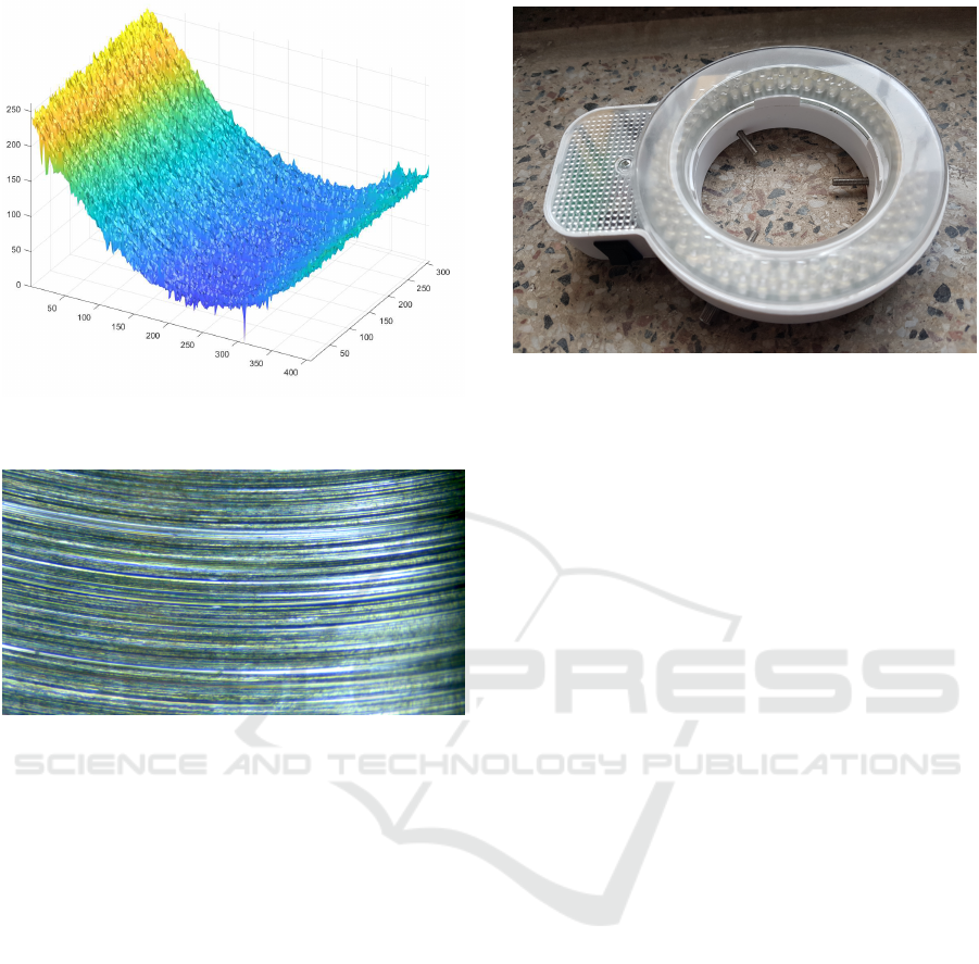
Figure 2: Samples of the surface scan of region №11 of part
№10.
Figure 3: Samples of the photo of region №16 of part №7.
are calculated from grey level co-occurrence matrix
(GLCM). This matrix can be calculated in various di-
rections and different distances relative to neighbour-
hood pixels. Then a set of features can be estimated
for a set of several GLMCs. These features describe
different statistical information of an image and they
are successfully used in the field of surface quality
control (Alegre et al., 2010) and other fields of image
processing (Chandraratne et al., 2006; Sabino et al.,
2004; Torabi et al., 2007). The biggest weakness of
the GLMC is that it has high computational complex-
ity.
Li Liu et al. (Liu et al., 2012) used generalized
local binary patterns (LBP) for texture classification.
Difference-based and intensity-based features were
extracted from local patches. Then they were com-
bined into joint histograms. The classification based
on these histograms showed good results on the chal-
lenging texture datasets.
A review of methods for prediction of surface
quality was made by several authors (Benardos and
Vosniakos, 2003; Lu, 2008). Texture features can be
successfully applied for prediction of surface quality.
Chen et al. (Chen et al., 2008) described a method of
Figure 4: Ring light source used in the research.
estimation of the surface roughness using grey level
co-occurrence matrix under the conditions of ambi-
ent light. Authors noticed that the ambient light af-
fects calculated features. A new multivariate-based
method was used to minimize the influence of the
ambient light. Furthermore, it is important to con-
sider the light direction and the quality of the light
used to obtain the surface images. In the previous re-
searches (Trambitckii et al., 2016) the correlation be-
tween texture features and roughness parameters was
estimated. Results of the research showed that ring
light can be a reliable light source for the tasks of
surface quality assessment using an industrial camera.
The main advantage of the ring light is its rotational
invariance.
In this research, a set of focus texture features
(listed in Chapter 4.2) is used to analyse the surface
quality of metal parts under the conditions of a ring
light source. The focus texture features were selected
for this research because such features can reflect and
deliver the information about a surface shape under
appropriate lighting conditions. Correlation coeffi-
cients between the texture features and a set of rough-
ness parameters (listed in Chapter 4.3), calculated for
the sample surfaces, is estimated. In contrast with the
previous researches (Trambitckii et al., 2016), where
the correlation was estimated for the same areas of
metal parts, in this paper the comparison of features
and parameters will be performed for different areas
of metal parts. Results of this research help to under-
stand, how the set of texture features can be used for
quick surface quality assessment.
3 DATA ACQUISITION
In this research, metal parts with cone-shaped sur-
faces were used (see Figure 1). The region of interest
ICPRAM 2019 - 8th International Conference on Pattern Recognition Applications and Methods
422

has the size around 1 mm ×1 mm. 3D surface rough-
ness was obtained with the Alicona 3D Infinite Focus
G4 measurement system. A lens with the magnifica-
tion of 20X was used. The lateral resolution (along
X- and Y-axis) of the measurement system with 20X
lens is 2.93 µm, the vertical resolution (along the Z-
axis) is around 100 nm. The sample of surface image
is shown in Figure 2.
2D images were obtained with a 2.23 MPix indus-
trial camera IDS UI-3360CP-C-HQ with an attached
telecentric macro lens. The camera has a resolution of
2048 px ×1088 px and the physical size of the sensor
is 2/3”. The macro lens attached to the camera has
a changeable magnification rate of 0.8X-4X. It gave
a possibility to make the region of interest similar to
the one obtained with 3D Alicona system. The aper-
ture of the lens cannot be stopped all the way down,
because of the strong decrease of sharpness caused
by diffraction. So the aperture was stopped about
halfway down to get the sharpest possible images and
a wider depth of field.
As was mentioned in the introduction, in optical
measurements of metal surfaces light plays an impor-
tant role because of the complex reflectance charac-
teristics of such surfaces. In this research, the ring
light source was used. The advantage of the ring light
is its rotation invariance of shadows of surface im-
ages relative to the lighting source. A sample image
of the surface obtained with a 2D camera is shown
in Figure 3. The ring light source used in this pa-
per is presented in Figure 4. The observed workpiece
area of the metal surface is a countersink. The cutting
speed of the tool, used to produce these drill hole, var-
ied from 175 to 185 m/min, to get a different level of
roughness. Thirteen metal parts were processed such
a way. For each part, it was taken about twenty 2D
images. It was measured the same amount of 3D data
for the same set of metal parts. This resulted in 250
2D images and 250 3D surfaces.
4 ESTIMATION OF
CORRELATION
4.1 Data Processing
For calculation of features and parameters, each im-
age and surface was cropped. Cropping removes ar-
eas of images near the edges. The edges are less sharp
than the centre areas. Also, Alicona 3D system and
IDS industrial camera have different aspect ratios. Af-
ter cropping 2D images and 3D surfaces both have the
same aspect ratio, which is necessary for the next cal-
Table 1: Amount of data for correlation estimation.
2D Images 3D Surfaces
Amount 250 250
Features/Parameters 27 10
culations.
In the next step, every image and surface is di-
vided into a grid of several subregions. Each feature
and parameter was calculated for every of such subre-
gions. The sizes of subregions were picked in such a
way that both output matrices had the same size. This
resulted in two equal-dimension sets of matrices: 2D
texture features and 3D roughness parameters. Then
the values of each matrix were averaged. These cal-
culations resulted in a set of 27 × 250 mean values of
texture features and 10 × 250 mean values of rough-
ness parameters. These values are presented in Ta-
ble 1.
4.2 Texture Features
27 different texture features were calculated in MAT-
LAB environment for a set of surface images, ob-
tained with the industrial camera. In this chapter, tex-
ture features which were used in this research are de-
scribed.
4.2.1 Histogram Entropy
(F
HEN
). It is a statistical feature of randomness that
can be used to characterize the texture of an image. It
is calculated by (C. Gonzalez et al., 2004; Firestone
et al., 1991):
F
HEN
= −
∑
k
(p
k
log
b
(p
k
)) , (1)
where k is the number of grey levels, b = 2 is the
base of the log function to express entropy in bits, and
p
k
is the probability that the grey level k occurs in
image:
p
k
=
h(k)
D
, (2)
where D is the number of pixels in the image.
4.2.2 Histogram Range
(F
HRA
). It is the difference between maximum grey
level and minimum grey level of an image (Firestone
et al., 1991):
F
HRA
= max(k|h(k) > 0) − min (k|h(k) > 0) , (3)
where h(k) is the value of the histogram h for the
k-th grey level.
Estimation of Correlation between Texture Features and Surface Parameters for Milled Metal Parts
423

4.2.3 Image Curvature
The grey level intensity of pixel (x, x) will be denoted
as g(x, y). If the grey levels are treated as a 3D surface
(x, y, g(x, y)), the curvature in a sharp image area is
expected to be higher than in an unsharp area (Helmli
and Scherer, 2001). The first step in calculating a fea-
ture, based on curvature, is to approximate the surface
f (x, y) = p
0
x + p
1
y + p
2
x
2
+ p
3
y
2
. The coefficients
P = (p
0
, p
1
, p
2
, p
3
)
t
are found using a least squares
approximation (Nayar et al., 1996) with g
0
and g
2
:
g
0
=


−1 0 1
−1 0 1
−1 0 1


, (4)
g
2
=


1 0 1
1 0 1
1 0 1


, (5)
P = (
g
0
∗ I
6
;
g
t
0
∗ I
6
;
3g
2
∗ I
10
−
g
t
2
∗ I
5
;−
g
2
∗ I
5
+
g
t
2
∗ I
10
)
t
.
(6)
Then these coefficients are combined in order to
form a texture feature. An experimental evaluation
(Helmli and Scherer, 2001) shows that the simple sum
of the absolute values results in an adequate focus
measure F
ICU
:
F
ICU
= |p
0
| + |p
1
| + |p
2
| + |p
3
| . (7)
4.2.4 Steerable Filter-based
A focus texture feature F
ST EF
is based on steerable
filters. Steerable filters represent a way to synthesize
filters of arbitrary orientation using a linear combi-
nation of basis filters. Such synthesis is used to de-
termine analytically the filter output as a function of
orientation (Minhas et al., 2009b).
4.2.5 Spatial Frequency
Let denote the number of horizontal and vertical pix-
els of the image as M and N, respectively. Frequen-
cies for rows and columns are defined by (M. Eski-
cioglu and S. Fisher, 1996):
RFreq =
v
u
u
t
1
M · N
M
∑
x=1
N
∑
y=1
|g(x + 1, y) − g(x , y)|
2
(8)
and
CFreq =
v
u
u
t
1
M · N
M
∑
x=1
N
∑
y=1
|g(x, y + 1) − g(x , y)|
2
.
(9)
Thus, spatial frequency F
SFR
is defined as
F
SFR
=
q
(RFreq)
2
+ (C Freq)
2
. (10)
4.2.6 Other Texture Features
Along with the listed texture features, also follow-
ing features were tested on the samples surfaces:
absolute central moment (Shirvaikar, 2004), Bren-
ner’s focus measure (Santos et al., 1997), image
contrast (Nanda and Cutler, 2001), image curvature
(Helmli and Scherer, 2001), DCT (discrete cosine
transform) energy (Shen and Chen, 2006), DCT en-
ergy ratio (Lee et al., 2009), Gaussian derivative
(Geusebroek et al., 2000), variance of grey-level
(Krotkov and Martin, 1986), local variance of grey-
level (Pech-Pacheco et al., 2000), normalized vari-
ance of grey-level (Santos et al., 1997), energy of
gradient (Subbarao et al., 1992), thresholded gradi-
ent (Santos et al., 1997), squared gradient (M. Eski-
cioglu and S. Fisher, 1996), Helmli’s measure (Helmli
and Scherer, 2001), histogram entropy (Krotkov and
Martin, 1986) and histogram range (Firestone et al.,
1991), energy of Laplacian (Subbarao et al., 1992),
modified Laplacian (Nayar et al., 1996), variance
of Laplacian (Pech-Pacheco et al., 2000), diagonal
Laplacian (Thelen et al., 2009), steerable filters-based
(Minhas et al., 2009a), spatial frequency (M. Eski-
cioglu and S. Fisher, 1996), Tenengrad (Krotkov and
Martin, 1986), Tenengrad variance (Pech-Pacheco
et al., 2000), Vollat’s correlation-based (Santos et al.,
1997), wavelet sum (Yang and Nelson, 2003) and
wavelet variance (Yang and Nelson, 2003).
4.3 Roughness Parameters
The surface quality can be estimated using roughness
parameters established in international standards (ISO
25178). In this research the following ISO roughness
parameters were used: S
a
(arithmetical mean devia-
tion of the assessed surface), S
q
(root mean square
deviation of the surface), S
sk
(skewness of the sur-
face), S
ku
(kurtosis of the surface), S
v
(maximum val-
ley height of the surface), S
p
(maximum peak height
of the surface), S
z
(maximum height of the surface,
i.e. the difference between the highest peak and the
deepest valley), S
dq
(root mean square surface slope)
and S
dr
(developed interfacial area ratio). Along with
the ISO parameters listed above another roughness
parameter from other source was used - S
sc
(mean
summit curvature) (Stout et al., 1994).
ICPRAM 2019 - 8th International Conference on Pattern Recognition Applications and Methods
424

0
0,1
0,2
0,3
0,4
0,5
0,6
0,7
0,8
0,9
1 9
17 25 33 41 49 57 65 73 81 89 97
105 113 121 129 137 145 153 161 169 177 185 193 201 209 217 225 233 241 249 257 265
Correlation
Coefficient
Pair №
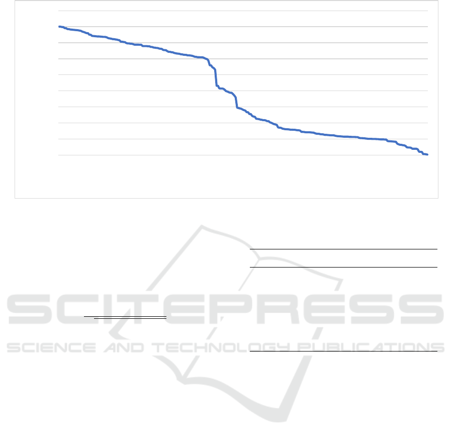
Figure 5: Correlation coefficient distribution between different pairs of texture features and roughness parameters.
4.4 Evaluation of Correlation
Having two variable sets of the same size, Pear-
son’s correlation coefficient can be estimated between
them:
ρ(a, b) =
∑
(a − ¯a)(b −
¯
b)
p
∑
(a − ¯a)
2
(b −
¯
b)
2
, (11)
where a, b are two input variables of the same size,
and ¯a,
¯
b are the averages of these variables.
The closer correlation coefficient is to 1 or -1, the
more linear dependency two variables have. If the
correlation coefficient is equal to 0, then there is no
linear dependency between them. If the correlation
coefficient is higher than 0, then such correlation is
called positive. If it is lower than 0, then the correla-
tion is called negative.
In our research, the correlation between both sets
of 2D texture features and 3D roughness parameters
was estimated. The correlation between 270 pairs (27
features × 10 parameters) of vectors was calculated.
Every feature and parameter vector has a length of
250 (equal to the amount of the sample images). The
distribution of the correlation for all pairs is shown in
Figure 5.
For correlation coefficient, an interpretation of the
Brosius criteria (Brosius, 1998) was used. These cri-
teria are listed in Table 2. This interpretation of the
correlation coefficients gives an easier explanation
whether values have a weak or strong correlation.
Table 2: Correlation coefficient interpretation.
Absolute value of coefficient Interpretation
0 no correlation
0 < ρ < 0, 2 very weak
0, 2 < ρ < 0, 4 weak
0, 4 < ρ < 0, 6 medium
0, 6 < ρ < 0, 8 strong
0, 8 < ρ < 1 very strong
1 perfect
5 RESULTS AND DISCUSSION
Previously in the work (Trambitckii et al., 2016) it
was mentioned, that a set of texture features, calcu-
lated for surfaces with removed waviness, has shown
weak correlation with 3D parameters. This phe-
nomenon can be explained. Texture features reflect
not only surface roughness, but also a low frequency
of the surface – waviness. When the correlation be-
tween texture features and roughness parameters is
estimated, waviness should not be removed from the
3D surfaces. Thus, in this research raw 3D surface
data was used for calculation of roughness parame-
ters.
In this research, the texture features calculated for
images of metal surfaces under ring light conditions
showed strong (up to 0.8009) correlation between the
roughness parameters.
The Pearson’s correlation coefficients between 27
texture features and 10 roughness parameters were
calculated. It resulted in the array of 270 pair-wise
Estimation of Correlation between Texture Features and Surface Parameters for Milled Metal Parts
425

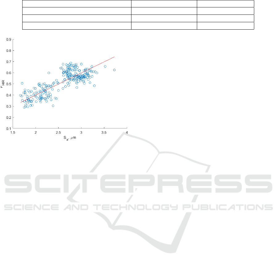
Table 3: Some correlation coefficients between several pairs.
Roughness parameter Texture feature Correlation coefficient
S
a
(arithmetical mean height of the surface) F
HRA
(histogram range) 0.8009
S
q
(root mean square height of the surface) F
ICU
(image curvature) 0.7915
S
z
(maximum height of the surface) F
HEN
(histogram entropy) 0.7826
Figure 6: Scatter plot of parameter pairs of the average sur-
face roughness (S
a
) and the histogram range (F
HIR
). Linear
regression (red line) was performed to get the relationship
between these two values. A correlation coefficient between
these parameters is equal to 0.8009.
correlation coefficients. For all the coefficients ab-
solute values were calculated, as some of the coeffi-
cients have negative values. Then all pairs were sorted
from the highest to the lowest values of the correla-
tion coefficients. A plot was created based on this
information. The plot shows the distribution of the
correlation coefficients for all 270 pairs, see Figure 5.
X-axis represents the absolute correlation coefficient
value. Y -axis is an index of the pair, sorted by the cor-
relation coefficient value in descending order. 40% of
feature/parameter pairs showed a strong (ρ > 0.6) cor-
relation. The correlation coefficients of several pairs
are listed in Table 3.
The performed research showed that under our
conditions the most correlated roughness parameters
are S
a
, S
q
, S
z
(see a description of the parameters in
Chapter 4.3). The most correlated texture features are
the histogram entropy, the histogram range, the im-
age curvature, the steerable filters-based and the spa-
tial frequency (see a description of these features in
Chapter 4.2). An example of the most correlated pair
(S
a
and the histogram range) is shown in Figure 6. An
average value of the correlation coefficient between
them is equal to 0.8009.
The future work can be focused on the calculation
of correlation among different texture features itself.
A larger set of parts can be produced to increase the
number of images in a dataset. More texture features
can be implemented to obtain probably even higher
correlation between features and parameters.
The performed research showed that there is a
strong correlation between texture features and rough-
ness parameters. This means that texture features can
be successfully applied to roughness assessment of
metal surfaces, as well as for the estimation of the
surface quality. This method of non-contact quality
control gives a possibility to find parts with certain
defects in a fast and reliable way on the basis of cost-
effective hardware equipment. It can help to increase
the rate of detection of parts, which are not fulfil given
requirements.
6 CONCLUSION
During the research, a set of 27 texture futures was
calculated for metal surface images. A set of 10
roughness parameters was calculated for the same
metal parts. The correlation between these sets was
estimated. 40% of feature/parameter pairs showed a
strong (ρ > 0.6) correlation. Thus, texture features
can reflect roughness information of a surface under
the controlled lighting conditions. It shows that tex-
ture features can be used to estimate metal surface
quality using images obtained with low-cost 2D cam-
eras.
ACKNOWLEDGEMENTS
The research project, which forms the basis of this pa-
per, is supported by the Thuringian Ministry of Econ-
omy, Employment and Technology (TMWAT) with
means from the European Social Fund (ESF). The re-
sponsibility for the content of this paper lies with the
author. Special thanks are due to the Society for Pro-
duction Engineering and Development Schmalkalden
(Germany), especially to Dr. Daniel Garten, for pro-
viding the measurement equipment and the processed
metal parts for the research.
ICPRAM 2019 - 8th International Conference on Pattern Recognition Applications and Methods
426

REFERENCES
ISO 25178: Geometric Product Specifications (GPS) Sur-
face texture: areal.
Alegre, E., Alaiz-Rodr
´
ıguez, R., Barreiro, J., Fidalgo,
E., and Fern
´
andez, L. (2010). Surface finish con-
trol in machining processes using haralick descrip-
tors and neuronal networks. In Computational Model-
ing of Objects Represented in Images, pages 231–241,
Berlin, Heidelberg. Springer Berlin Heidelberg.
Benardos, P. and Vosniakos, G.-C. (2003). Predicting sur-
face roughness in machining: a review. 43:833–844.
Brosius, F. (1998). SPSS 8. International Thomson Publish-
ing.
C. Gonzalez, R., E. Woods, R., and L. Eddins, S. (2004).
Digital Image Processing Using Matlab, volume 1.
Chandraratne, M., Samarasinghe, S., Kulasiri, D., and Bick-
erstaffe, R. (2006). Prediction of lamb tenderness us-
ing image surface texture features. 77:492–499.
Chen, Z., Zhang, Z., Shi, J., Chen, R., Huang, R., and
Zhang, C. (2008). A multivariate method for surface
roughness vision inspection in different ambient light.
In 2008 IEEE International Conference on Mecha-
tronics and Automation, pages 324–328.
Firestone, L., Cook, K., Culp, K., Talsania, N., and Jr., K. P.
(1991). Comparison of autofocus methods for auto-
mated microscopy.
Geusebroek, J.-M., Cornelissen, F., Smeulders, A. W.,
and Geerts, H. (2000). Robust autofocusing in mi-
croscopy. Cytometry: The Journal of the International
Society for Analytical Cytology, 39(1):1–9.
Haralick, R. M., Shanmugam, K., and Dinstein, I. (1973).
Textural Features for Image Classification. IEEE
Transactions on Systems, Man, and Cybernetics,
SMC-3(6):610–621.
Helmli, F. S. and Scherer, S. (2001). Adaptive shape from
focus with an error estimation in light microscopy. In
ISPA 2001. Proceedings of the 2nd International Sym-
posium on Image and Signal Processing and Analysis.
In conjunction with 23rd International Conference on
Information Technology Interfaces (IEEE Cat., pages
188–193.
Krotkov, E. and Martin, J.-P. (1986). Range from focus.
In Robotics and Automation. Proceedings. 1986 IEEE
International Conference on, volume 3, pages 1093–
1098. IEEE.
Lee, S.-Y., Yoo, J.-T., Kumar, Y., and Kim, S.-W. (2009).
Reduced energy-ratio measure for robust autofocus-
ing in digital camera. IEEE Signal Processing Letters,
16(2):133–136.
Liu, L., Zhao, L., Long, Y., Kuang, G., and Fieguth, P.
(2012). Extended local binary patterns for texture
classification. Image Vision Comput., 30(2):86–99.
Lu, C. (2008). Study on prediction of surface quality in
machining process. Journal of Materials Processing
Technology, 205(1):439 – 450.
M. Eskicioglu, A. and S. Fisher, P. (1996). Image quality
measures and their performance. 43:2959 – 2965.
Minhas, R., Mohammed, A. A., Wu, Q. J., and Sid-Ahmed,
M. A. (2009a). 3d shape from focus and depth map
computation using steerable filters. In International
Conference Image Analysis and Recognition, pages
573–583. Springer.
Minhas, R., Mohammed, A. A., Wu, Q. M. J., and Sid-
Ahmed, M. A. (2009b). 3d shape from focus and
depth map computation using steerable filters. In
Kamel, M. and Campilho, A., editors, Image Analysis
and Recognition, pages 573–583, Berlin, Heidelberg.
Springer Berlin Heidelberg.
Nanda, H. and Cutler, R. (2001). Practical calibrations for a
real-time digital omnidirectional camera. CVPR Tech-
nical Sketch, 20:2.
Nayar, S. K., Watanabe, M., and Noguchi, M. (1996). Real-
time focus range sensor. IEEE Transactions on Pat-
tern Analysis and Machine Intelligence, 18(12):1186–
1198.
Pech-Pacheco, J. L., Crist
´
obal, G., Chamorro-Martinez, J.,
and Fern
´
andez-Valdivia, J. (2000). Diatom autofocus-
ing in brightfield microscopy: a comparative study.
In Pattern Recognition, 2000. Proceedings. 15th In-
ternational Conference on, volume 3, pages 314–317.
IEEE.
Sabino, D. M. U., da Fontoura Costa, L., Gil Rizzatti,
E., and Antonio Zago, M. (2004). A texture ap-
proach to leukocyte recognition. Real-Time Imaging,
10(4):205–216.
Santos, A., Ortiz de Sol
´
orzano, C., Vaquero, J. J., Pena, J.,
Malpica, N., and Del Pozo, F. (1997). Evaluation of
autofocus functions in molecular cytogenetic analysis.
Journal of microscopy, 188(3):264–272.
Shen, C.-H. and Chen, H. H. (2006). Robust focus mea-
sure for low-contrast images. In Consumer Electron-
ics, 2006. ICCE’06. 2006 Digest of Technical Papers.
International Conference on, pages 69–70. IEEE.
Shirvaikar, M. V. (2004). An optimal measure for camera
focus and exposure. In System Theory, 2004. Proceed-
ings of the Thirty-Sixth Southeastern Symposium on,
pages 472–475. IEEE.
Stout, K., Sullivan, P., Dong, W., Mainsah, E., Luo, N.,
Mathia, T., and Zahouani, H. (1994). Development of
Methods for Characterisation of Roughness in Three
Dimensions. Publication No. EUR 15178 EN of the
Commission of the European Communities, Luxem-
bourg.
Subbarao, M., Choi, T.-S., and Nikzad, A. (1992). Focusing
techniques. In Machine Vision Applications, Architec-
tures, and Systems Integration, volume 1823, pages
163–175. International Society for Optics and Photon-
ics.
Thelen, A., Frey, S., Hirsch, S., and Hering, P.
(2009). Improvements in shape-from-focus for holo-
graphic reconstructions with regard to focus operators,
neighborhood-size, and height value interpolation.
IEEE Transactions on Image Processing, 18(1):151–
157.
Torabi, M., Ardekani, R., and Fatemizadeh, E. (2007). Dis-
crimination between alzheimer’s disease and control
group in mr-images based on texture analysis using
artificial neural network.
Estimation of Correlation between Texture Features and Surface Parameters for Milled Metal Parts
427

Trambitckii, K., Anding, K., Polte, G., and Garten, D.
(2014). Elimination of out-of-focus regions for sur-
face analysis in 2-d colour images.
Trambitckii, K., Anding, K., Polte, G., Garten, D., Musal-
imov, V., and Kuritcyn, P. (2016). The application of
texture features to quality control of metal surfaces.
ACTA IMEKO, 5(4):19–23.
Yang, G. and Nelson, B. J. (2003). Wavelet-based aut-
ofocusing and unsupervised segmentation of micro-
scopic images. In Intelligent Robots and Systems,
2003.(IROS 2003). Proceedings. 2003 IEEE/RSJ In-
ternational Conference on, volume 3, pages 2143–
2148. IEEE.
ICPRAM 2019 - 8th International Conference on Pattern Recognition Applications and Methods
428