
Categorical Modeling Method, Proof of Concept for the Petri Net
Language
Daniel-Cristian Crăciunean
Computer Science and Electrical Engineering Department, Lucian Blaga University of Sibiu,
Bulevardul Victoriei 10, 550024 Sibiu, Romania
Keywords: Modeling Method, Metamodel, Category Theory, Functors, Natural Transformation, Limit, Colimit,
Categorical Modeling Method.
Abstract: Modeling increases the importance of processes significantly, but also imposes higher requirements for the
accuracy of process specifications, since an error in the design of a process may only be discovered after it
already produces large cumulative losses. We believe that modeling tools can help build better models in a
shorter time. This inevitably results in the need to build formal models that can be theoretically verified.
A category as well as a model is a mixture of graphical information and algebraic operations. Therefore,
category language seems to be the most general to describe the models. The category theory offers an
integrated vision of the concepts of a model, and also provides mechanisms to combine models, mechanisms
to migrate between models, and mechanisms to build bridges between models. So, category theory simplifies
how we think and use models. In this paper we will use the language offered by the category theory to
formalize the concept of Modeling Method with the demonstration of the Categorical Modeling Method
concept for the Petri Net grammar.
1 INTRODUCTION
Nowadays, modeling is the main engine for
increasing business process performance. But the
modeling of business processes has led to dramatic
changes in the organization of work and has allowed
new ways of doing business. Therefore, process
modeling has become an extremely important factor
in increasing company performance. As a result,
process models are widely used in organizing and
managing companies.
There are very general models such as: operations
management and, in particular, operational research,
which have standard solutions, but business processes
are very diverse so that metamodels have to be built
ad-hoc.
If the operations management can be based on
standard immutable models with precise semantics
such as linear programming, queueing models,
Markov chains, etc. process models in BPM typically
serve multiple purposes and are more heterogeneous.
Therefore, making a good BPM model is a hard
task especially if the modeling tool is not appropriate.
It is not easy to make good process models within
a reasonable time. However, process models are very
important. We believe that modeling tools can help
build better models in a shorter time.
The purpose of a process model is to decide what
tasks to perform and in what order. Activities may be
sequential, parallel or concurrently, may also be
optional or mandatory, and the execution of some
activities may be repetitive.
The best known process model is the transition
system. A transition system consists of states and
transitions. Any process model with executable
semantic can be mapped to a transition system.
Transition systems are simple but cannot efficiently
express concurrency. For example, if we have a
system with n parallel activities that can be executed
in any order then there is n! possible execution
sequences. The transition system therefore requires 2
n
states and n×2
n-1
transitions (van der Aalst, 2011).
Given the concurrency nature of business
processes, more expressive models such as Petri Nets,
BPMN, EPC and UML are needed to make them
more concise and legible. Many features defined for
transition systems can easily be translated into these
top-level mechanisms.
All these process models have in common that
processes are described in terms of activities (and
possibly subprocesses). The ordering of these
Cr
˘
aciunean, D.
Categorical Modeling Method, Proof of Concept for the Petri Net Language.
DOI: 10.5220/0007360602810289
In Proceedings of the 7th International Conference on Model-Driven Engineering and Software Development (MODELSWARD 2019), pages 281-289
ISBN: 978-989-758-358-2
Copyright
c
2019 by SCITEPRESS – Science and Technology Publications, Lda. All rights reserved
281

activities is modeled by describing casual
dependencies.
The main concepts used in processes modeling
are: case, task, routing (van der Aalst and van Hee,
2004).
The life cycle of a case in a process represents the
routing of the case. Routing on certain branches is
based on four basic constructions that determine what
tasks must be performed and in what order (van der
Aalst and van Hee, 2004):
The behavior of a case is defined by a process and
therefore has a finite life, with a beginning that marks
the occurrence of a case, and an end that marks the
completion of the case.
Most of the times, the formalization of workflow
patterns is based on the graph theory. We will use in
this paper the category theory for this purpose.
A category as well as a model is a mixture of
graphical information and algebraic operations.
Therefore, category language seems to be the most
general to describe the models
The category theory works with patterns or forms
in which each of these forms describe different
aspects of the real world. Category theory offers both,
a language, and a lot of conceptual tools to efficiently
handle models.
Generally, building a model begins with an
informal model, used for discussion and
documenting, and ends with an executable model
useful for analyzing, simulating, or actually executing
the process.
Informal models are easy to understand but suffer
from ambiguity, while executable models are too
detailed to be easy to understand by all the parties
involved in building the model.
This conflict (dichotomy) between the informal
and the executable model largely reflects a certain
incompatibility between the metamodel and the
modeled object, and therefore is mainly due to the
insufficient alignment between the metamodel and
reality.
Due to the very large diversity of real world
processes, it is impossible for an existing metamodel
of a process to be well aligned in all cases.
This problem is often solved by endlessly adding
new facilities to existing metamodels to cover the
modeling requirements of processes that were not
foreseen in the initial phase. Obviously, these
additions lead to complicated metamodels, difficult to
understand and difficult to learn by those who are
going to use them.
Hence the need to build specific metamodels for
each domain that are totally compatible with the
specific processes of a given field.
2 THEORETICAL
FOUNDATIONS AND NOTES
Definition 1. (Manes, 1986; Barr and Wells, 2012) A
category is defined as follows: We consider a
collection of objects A, B, .. X, Y, Z, ... which we
denote by ob() and we call it the set of objects of .
For each pair of objects (X,Y) of , we consider a set
of arrows from X to Y denoted by (X,Y). On the set
of arrows we consider a composing operator denoted
by ∘, which attaches to each pair of arrows (f,g) of the
form: f:XY, g:YZ a morphism g∘f:XZ and
respecting the axioms 1 and 2.
1. The composition is associative:
If f:XY, g:YZ and
h:ZW(h∘g)∘f=h∘(g∘f):XW.
2. For each object X, there is the identity arrow
id
X
:XX with the property that id
X
∘f=f, g∘id
X
=g
for all pairs of arrows f:XY and g:UX.
Definition 2. (Barr and Wells, 2012; Walters, 2006)
Let and be two categories, a functor from to
consists of the functions:
ob
:ob( )ob(), and
for each pair of objects A, B of we have the
functions:
A,B
:(A,B)((A),(B)) which fulfills
the following conditions:
(1
A
)=1
(A)
, (fg) = fg if A
1
→ A
2
→A
3
.
Typically, all functions
ob
,
A,B
are denoted by the
symbol, for simplicity.
Definition 3. (Barr and Wells, 2012; Walters, 2006)
Let , be functors from category to category .
A morphism from to , also called natural
transformation, is a family of arrows in :
A
:AA (A ). So, for any arrow f:A B in ,
we have (f)∘
A
=
B
∘(f). This condition is called the
naturality condition.
Definition 4. (Barr and Wells, 2012; Barr and Wells,
2002) Let and be two graphs. A diagram in of
the graph is a functor: D: . is called the
shape graph of the diagram D.
Definition 5. (Barr and Wells, 2012; Barr and Wells,
2002) Let be a graph and a category. Let D:
be a diagram in with the form and
C
: be a
constant functor (which maps all objects in C and all
arcs in id
C
). A commutative cone with base D and
vertex C is a natural transformation p:
C
D.
Definition 6. The set of cones along with the
morphisms between them form a category that we call
the category of cones. A terminal object (cone) in the
MODELSWARD 2019 - 7th International Conference on Model-Driven Engineering and Software Development
282

category of cones, if any, is called a limit of the D
diagram. This limit is also called universal cone.
Definition 7. (Barr and Wells, 2012; Barr and Wells,
2002) Let be a graph and a category. Let D:
be a diagram in with the shape and
C
:
constant functor (which maps all objects in C and all
arcs in id
C
). A commutative cocone with base D and
vertex C is a natural transformation p:D
C
.
Definition 8. The set of cocones along with the
morphisms between them form a category we call the
category of cocones.
Definition 9. An initial object (cocone) in the
category of cocones, if any, is called colimit of
diagram D. This colimit is also called the universal
cocone.
Definition 10. (Barr and Wells, 2012; Barr and Wells,
2002) A sketch = (, , ,) consists of a graph
, a set of diagrams in , a set of cones in , and
a set of cocones in . The graph arrows of a sketch
are often called sketch operations.
Definition 11. (Barr and Wells, 2012; Barr and Wells,
2002) A model of a sketch =(,,,) is a functor
M from to Set that takes each diagram from to a
commutative diagram in Set, each cone from to a
cone limit and every cocone from to a colimit
cocone.
We will denote with numbers the nodes of the shape
graph, with lowercase letters the nodes of the graph
of sketches and with uppercase letters, the objects of
the categories.
3 CATEGORICAL SKETCH OF
THE MODELING METHOD
A model is a point of view over a domain. To be able
to perceive the purpose of this paper, it is important
to understand the term modeling method
(Karagiannis and Kühn, 2002), and the difference
between a modeling language and a modeling
method.
A modeling method consists of two components:
(1) a modeling technique, which is divided in a
modeling language and a modeling procedure, and (2)
mechanisms & algorithms working on the models
described by a modeling language (Karagiannis and
Visic, 2011).
The static part of a process model is a graph with
some syntactic restrictions (Karagiannis and
Junginger and Strobl, 1996). These restrictions will
then be introduced into the sketch of a modeling
method metamodel based on mechanisms specific to
the category theory such as commutative diagrams,
limits and colimits. The result is the concept of
Categorical Modeling Method.
In this paper we will define and demonstrate the
concept of Categorical Modeling Method for the Petri
Net grammar. A Petri Net is a type of transition
system in which a transition does not affect a global
state, but the occurrence of an event affects only a
subset of conditions in its neighborhood.
Also, Petri Nets are an established model of
parallel computing (Glynn, 2009). In addition,
expressive graphics determine a wide use of Petri
Nets in modeling, analysis and design, covering a
significant area of sequentially controlled processes,
from the dynamics of individual entities, to the
dynamics of some collective entities.
The static part of a Petri Net is a directed graph,
weighted and bipartite graph, i.e. consisting of two
types of nodes, called places, and transition
respectively. Oriented arcs combine either a place
with a transition or a transition with a place. There are
no arcs connecting two places between them, or two
transitions between them. As graphical
representation, places are represented by circles, and
transitions through bars or rectangles.
The dynamic part of a Petri Net is represented by
the distribution of tokens on the nets places and the
modification of this distribution by conditional
triggering of the transitions.
The edges can be labeled with weights that are
positive and integer values. If the weight is one, it is
usually omitted in the graphical representations.
Frequently, concepts of conditions and events are
used, places are conditions, and transitions are events.
A transition (event) possesses a number of input
places called preconditions and a number of output
positions, which are postconditions for the event in
question.
A transition is triggered if all preconditions and
all postconditions are met. The triggering of a
transition affects only the conditions of its neighbor,
i.e. its preconditions and postconditions.
From a syntactic point of view, a Petri Net can be
defined as follows:
Definition 13. A Petri Net (PN) is a directed graph
= (X,, , ) which satisfies the following properties:
1. is a bipartite graph: X=PT , PT=
where: P- is a finite set of places, T- is a finite set of
transitions .
2. is a finite set of arcs, divided into two subsets:
=
PT
TP
,
PT
TP
=,
Categorical Modeling Method, Proof of Concept for the Petri Net Language
283

3. , : X; are functions that associate to each
arc a source and a target. We will use the following
notations:
PT
=/
PT
,
TP
=/
TP
,
PT
=/
PT
,
TP
=/
TP
,
4. is a connected graph.
5. There is only one arc between any two nodes.
A place p∈P is an input place for a transition q∈T if
and only if there is a directed arc a
PT
so that (a)=p
and (a)=q. The set of input places in the transition q
is denoted with
.
A place p∈P is an output place for a transition q∈T
if and only if there is a directed arc a
TP
so that
(a)=q and (a)=p. The set of the output places of the
transition q is denoted with
.
A transition q∈T is an input transition for a place
p∈P if and only if there is a directed arc a
TP
so that
(a)= q and (a)=p. The set of input transitions in the
place p is denoted with
.
A transition q∈T is an output transition for a place
p∈P if and only if there is a directed arc a
PT
so that
(a)=p and (a)=q. The set of output transitions from
p is denoted with
.
Let's build the sketch corresponding to Petri Net.
We obviously start from the general sketch
corresponding to a directed multigraph with loops and
introduce the restrictions in the Petri Net definition
from above.
1. G is a bipartite graph: X=P⊔T. That is, the set of
objects X is the disjoint union of two subsets of
object P and T. This means that X is the coproduct
of a discrete diagram formed by two nodes and
with the vertex X, which in Set will become the
colimit of this discrete diagram. This discrete
diagram is reflected in the graph of the sketch as
in Figure 1.
2. is a set of arcs divided into two subsets =
pt
⊔
tp
. Therefore, the set of arcs is the disjoint
union of the two subsets of arcs
pt
and
tp
. This
means that is the coproduct of a discrete
diagram formed by two nodes. This discrete
diagram is reflected in the graph of the sketch as
in Figure 1.
3 , : X are functions that associate to an arc,
a source and a target. The additional notations
pt
,
tp
,
pt
and
tp
will also be reflected in the graph
of the sketch (Figure 1) because they are operators
of the sketch.
4 G is a connected graph. For this we will put the
condition that the pushout of with to be a
terminal object in the Set category.
5 There is only one arc between any two nodes. To
impose this constraint we will build the XX
product. This is the limit of a discrete diagram
formed by two nodes. The condition that is
required in this commutative diagram to have no
more than one arc between any two nodes is that
the function becomes a monomorphism in Set
(Figure 1). But is a monomorphism if and only
if the pullback of with exists and is equal to .
We have seen that a sketch = (, , , ) consists
of a graph , a set of diagrams in , a set of cones
in , and a set of cocones in .
Graph (Figure 1) has 8 nodes and 15 arrows.
These will be interpreted in a model as follows: (1) x
- all object X in a Petri Net model; (2) T
- all
transactions objects T from a Petri Net model; (3) P
-
all places objects P from a Petri Net model; (4) xx -
the Cartesian product of the set X with X; (5)
represents a terminal object in Set; (6) - represents
all relations between the objects of the model; (7)
pt
- represents the subset of relations
PT
that links
places with transactions; (8)
tp
- represents the subset
of relations
TP
that links transactions with places.
We have numbered these nodes to refer to them in the
shape graph of the diagrams.
Figure 1: The graph of the PN sketch.
The constraints will be imposed by commutative
diagrams, cones and cocones (Barr and Wells, 2012)
as follows.
1. The sketch will contain a commutative diagram.
The condition that a model does not contain more
than one arrow between two objects is ensured by
the injectivity of a function :XX. The shape
graph of this diagram is in Figure 2. The functor
d
1
is defined as follows: d
1
(6)=; d
1
(1)=x;
d
1
(4)=xx; d
1
(1’)=x; d
1
()=;d
1
()=; d
1
()=;
d
1
(
1
)=
1
; d
1
(
2
)=
2
.
MODELSWARD 2019 - 7th International Conference on Model-Driven Engineering and Software Development
284
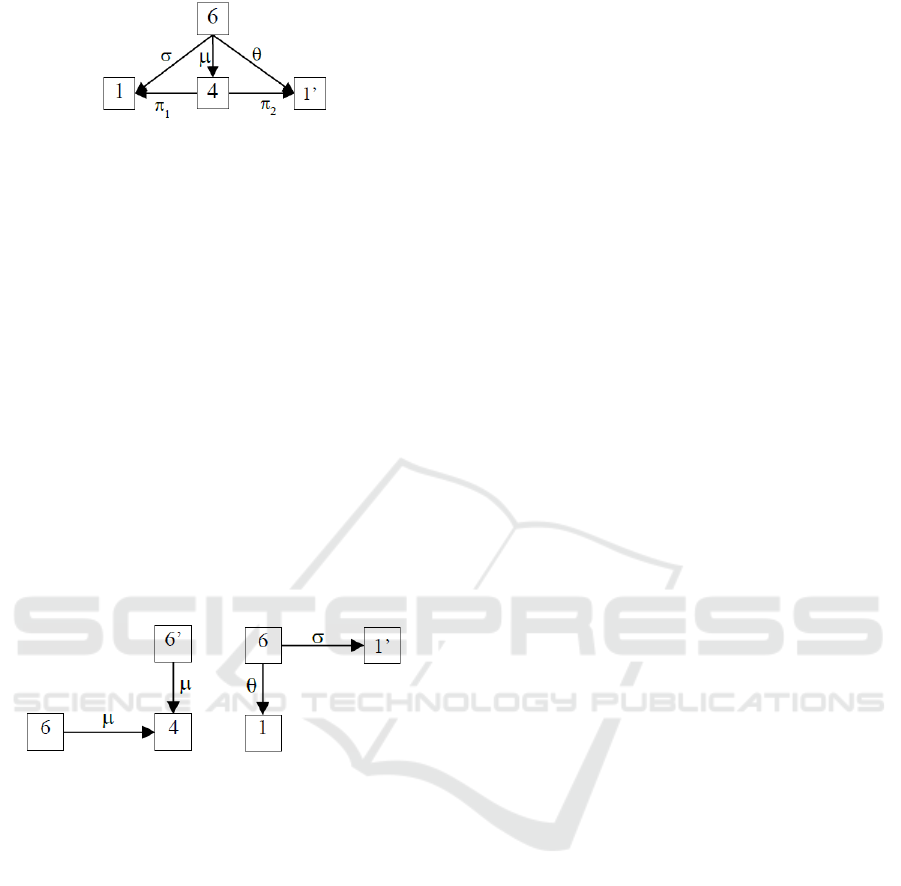
Figure 2: Shape graph of the commutative diagram.
2. The set of cones consists of the following:
The node denoted by xx in the graph of the
sketch will have to become the Cartesian product
XX in the Set category. For this, it will have to
be the limit of the discrete diagram with the shape
graph given by nodes 1 and 1'. The functor l
1
corresponding to this diagram will be defined as:
l
1
(1)=x; l
1
(1’)=x, and XX will be the limit of this
discrete diagram, i.e. the Cartesian product XX.
The node denoted with in the graph will become
the limit of a cone with an empty base, i.e. a
terminal object from Set.
At point v) the pullback of with is the limit of
the diagram l
2
. The shape graph of this diagram is
in Figure 3. and the functor l
2
corresponding to
this diagram is defined as: l
2
(6)=; l
2
(6’)=;
l
2
(4)=xx; l
2
()=. The limit of this diagram in
the Set category will have to be .
Figure 3: Shape graph of
pullback diagram.
Figure 4: Shape graph of
pushout diagram.
3. The set of cocones consists of the following:
At point i) X=P⊔T, i.e. X is the colimit of the
discrete diagram formed by the nodes p and t. The
shape graph of this diagram is made up of nodes 3
and 2 and the functor k
1
corresponding to this
diagram is defined as: k
1
(3)=p; k
1
(2)=t. Therefore,
the node denoted with x in the graph of the sketch
will become in the Set category the set X of all
objects involved in the model and will be the
colimit to this discrete diagram, i.e. the disjunctive
union of the P and T sets.
At point ii) =
PT
⊔
TP
, i.e. X is the colimit of the
discrete diagram formed by nodes
pt
and
tp
. The
shape graph of this diagram is made up of nodes 7
and 8 and the functor k
2
corresponding to this
diagram is defined as: k
2
(7)=
pt
; k
2
(8)=
tp
.
Therefore, the node denoted with in the graph of
the sketch will become in the Set category the set
which will be the colimit of this discrete
diagram.
At point iv) the pushout of with is a terminal
object. The condition that this colimit is a terminal
object in Set assures us that the graph G is
connected. The shape graph of this diagram is in
Figure 4. and the functor k
3
corresponding to these
diagram is defined as follows: k
3
(6)=; k
3
(1)=x;
k
3
(1’)=x; k
3
()=; k
3
()=.
So we’ve got the sketch of a Petri Net, we denote it
with L
1
(PN)=(, , ,).
4 THE METAMODEL
A model M of a sketch L
1
=(,,,) in the Set
category is a functor from to Set that takes each
diagram in to a commutative diagram, each cone in
to a cone limit and each cocone in to a cocone
colimit.
From the way we constructed the sketch L
1
(PN) it
follows that any model of the sketch L
1
(PN) in Set is
a Petri Net in the sense of the definition 13 and any
Petri Net in the sense of the definition 13 may be a
model of this sketch.
The sketch L
1
is the basic sketch of a modeling
method. The nodes of this sketch represent the types
of objects that can be defined in this modeling method
as well as the types of relations that can be defined
between these objects in this modeling method and
the arcs are the sketch operators.
Therefore these concepts will have to be
represented in the modeling tool on PaletteDrawers to
be used when visually building a model. Therefore we
consider a model of the sketch L
1
, :L
Sets
which associates to each class (node) from L
1
with an
instance of that class. These objects will be put into
PaletteDrawers for use when visually building a
model. In PaletteDrawers are only the necessary
entities for use when visually building a model.
For Petri Net, in sketch L
1
(PN) the basic concepts
that will be put in the PaletteDrawers for use when
visually building a model will have the type indicated
by the vertex of the sketch from Figure 1.
PaletteDrawers will contain only the following
entities: (p),(t),(
pt
) and (
tp
). Therefore,
PaletteDrawers will be populated with four elements.
Any model of the sketch L
1
=(,,,) is a
concrete model that complies with the conditions
imposed by the sketch L
1
. To construct such a model,
it is sufficient to consider a model H
:L
Sets that
Categorical Modeling Method, Proof of Concept for the Petri Net Language
285
associates the classes (nodes) in the sketch L
1
with
sets of extensions of these classes.
For Petri Net the model H
:L
Sets becomes:
H
p)=P is the set of all extensions of type place in a
Petri Net model; H
t)=T is the set of all extensions
of type transition in a Petri Net model; H
pt
)=
PT
represents the subset of relations
PT
; H
tp
)=
TP
represents the subset of relations
TP
; The other
objects and arcs of the sketch are useful for imposing
constraints on the model. The arrows of the graph will
be interpreted as functions with the same name as the
domains corresponding to the model image H
2
.
Let H
and H
be two models of the sketch L
1
defined as above. Then we can define a natural
transformation :H
H
. It is obvious that there isn’t
always a natural transformation between two models
and it is equally obvious that there are models among
which we have such transformations.
Therefore, the set of models H
, k0 together with
the natural transformations between models form a
category that we call the category of specifiable
models in a Modeling Method. Each object in this
category is a specifiable model in a Modeling
Method, represented by the sketch L
1
.
The natural transformations in the category of
specifiable models in a Modeling Method transfers
the properties of a Model to another Model, and can
be the basis for model comparison.
5 THE DYNAMIC BEHAVIOR OF
MODELS
The dynamic behavior of a system over time is
modeled by procedures. The simulation begins by
initializing the system with data that describe its
initial state. The dynamics of the system is
accomplished through the succession of procedures
being executed.
In the concept of modeling method, simulation of
a model is based on mechanisms and algorithms that
are written in an imperative programming language.
The behavior of the model is based on the state idea,
determined by the values of the variables.
Transitions will look like (V
k
,
k
, V
k+1
) where V
k
is the state vector of the system before the transition,
V
k+1
is the state vector of the system at the end of the
transition, and
k
is a process represented by natural
transformation.
On the other hand, executing a transition changes
an instance of the model by turning it into another
instance. As a result, we will use transitions of the
form (
1
, p,
2
) where
1
is the instance of the model
before the execution of the functions p and
2
is the
instance of the same model after executing the
functions p.
Let H
2
be a model of the Petri Net sketch, L
1
defined as above, i.e. an object of the Petri Net
category. We denote with L
2
this model L
2
= H
2
(L
1
).
The L
2
model represents a concrete Petri Net. The
object X of this model is a set of classes of type
transitions or places; T is a set of classes of
transitions, P is a set of classes of type places.
The object is a set of relation types that can be
defined between these entities.
The arcs of the sketch indicate between what types
of objects the corresponding relations can be
established. That is, L
2
contains all types of objects
specific to the Petri Net considered.
Referring to Petri Net example to create the
instances of the model L
2
, it is sufficient to limit
ourselves to the elements in the subsketch which
contain all the necessary information to use the model
and which are: P,T,
PT
and
TP
. The other objects and
arcs of the sketch are useful for imposing the syntactic
constraints on the model.
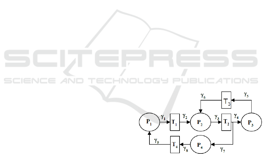
If in the above model we have:
T={T
1
,T
2
,T
3
,T
4
} is a set of classes of type
transitions;
P={P
1
,P
2
,P
3
,P
4
} is a set of classes of type places;
PT
={
1
,
3
,
5
,
8
} is a set of classes of type
relation from P to T.
TP
={
2
,
4
,
6
,
7
,
9
} is a set of classes of type
relation from T to P.
Figure 5: Petri-Net model example.
TP
:
TP
T, associates to each relation from
TP
the source node from T:
TP
(
2
)= T
1
;
TP
(
4
)= T
2
;
TP
(
6
)= T
3
;
TP
(
7
)= T
2
;
TP
(
9
)= T
4
;
TP
:
TP
P, associates to each relation from
TP
the source node from P:
TP
(
2
)= P
2
;
TP
(
4
)= P
3
;
TP
(
6
)= P
2
;
TP
(
7
)= P
4
;
TP
(
9
)= P
1
;
PT
:
PT
P, associates to each relation from
PT
the source node from P:
PT
(
1
)= P
1
;
PT
(
3
)= P
2
;
PT
(
5
)= P
3
;
PT
(
8
)= P
4
;
MODELSWARD 2019 - 7th International Conference on Model-Driven Engineering and Software Development
286

PT
:
PT
T, associates to each relation from
PT
the source node from T:
PT
(
1
)= T
1
;
PT
(
3
)= T
2
;
PT
(
5
)= T
3
;
PT
(
8
)= T
4
;
then the PN model is like in Figure 5.
We consider an instance functor defined on such
a model with values in the Set category:
: L
Sets
Which associates to each set of classes in L
2
a set
of instances, i.e. each class will be replaced by one
instance of it.
In our case, the instances differ from one another
by the number and positioning of tokens on the Petri
Net instance arcs, i.e. by the state corresponding to
each instance.
If we have two models ,:L
Sets then we can
define a natural transformation :.
The set of all models together with all the natural
transformations between them form a category that
we call the category of instances and natural
transformations of the L
2
model and we denote it with
CIT.
We observe that in this case natural
transformations become functors, i.e. it transforms
objects into objects and arcs in arcs while retaining
the structure.
The state of the Petri Net is characterized by the
distribution of tokens on the nets places. The dynamic
behavior of a system is represented by state changes
that are subject to transaction triggering rules. As
detailed below, there are rules for triggering different
transactions for different classes of Petri Nets
(Weske, 2012).
The marking (or state) of a Petri Net is defined by
a function M:P → N which associates places of a Petri
Net with natural numbers representing the number of
tokens found in each place of the net. Generally, a
marking (a subset of conditions) formalizes a global
state notion by specifying the conditions that are met
at one time.
If the arcs are ordered entirely by their identifier
(such as in p
1
, p
2
, p
3
, p
4
) the state can be expressed by
a vector. In our case through the vector M=[1, 0, 0, 0]
for example.
The state of each place p
i
will be given by an
attribute with integer values of the corresponding
class that we denote as p
i
.State. This means that the
state of an instance of the chosen Petri Net model is
represented by the vector M=[ p
1
.State, p
2
.State,…,
p
n
.State] where n is the total number of places of the
Petri Net model. We will also denote the state of a
place p.State with M(p).
Therefore, an instantiation functor :L
Sets will
create an instance of the model L
2
that will have a
certain state represented by a marking M=[ p
1
.State,
p
2
.State,…, p
n
.State] with the meaning from above.
In this context, a set of Petri Net classes have been
introduced, which differ from each other by their
triggering behavior and the structure of their tokens.
We will address only two of them: Condition Event
Nets and Place Transition Nets (Weske, 2012).
Condition Event Nets (Weske, 2012) make up the
fundamental class of Petri Nets. A Petri Net is a
Condition Event Net if p.State≤1 for all places p∈P
and for all states M.
Place Transition Nets are an extension of the
Condition Event Nets, so there may be an arbitrary
number of tokens in any Petri Net place. Additionally,
multiple tokens can be consumed from an input place,
and multiple tokens can be produced at the output
places when triggering a transition, based on the
weight associated with the arcs connected to the
transition. This extension can be represented
graphically by multiple arcs from a particular entry
place to a transition or with arcs labeled with natural
numbers to mark their weight.
A Petri Network is a Place Transition Nets
(Weske, 2012), if it has a function w:→N that
associates each arc with a weight (capacity).
The dynamic behavior of a Place Transition Net is
defined as follows: A transition t is triggered if and
only if each input place p of the transition t contains
at least the number of tokens defined by the weight of
the link arc, i.e. if M(p) ≥ w(p , t).
When a transition t is triggered, the number of
chips withdrawn from its input places and the number
of tokens added to its outputs are determined by the
weights of the arcs.
For the transition t, from each input place p, w(p,t)
tokens are withdrawn, and to each output place q are
added w(t,q) tokens.
The triggering of a transition t in a state
transforms the state M into a state M’, as follows:
(∀p ∈
-1
t) M
’
(p) = M (p) - w (p, t) ∧ (∀p ∈
1
t ) M
’
(p)
= M (p) + w (t, p).
If we consider that each instance has a global state
specified by the vector M
k
, then a process execution
modeled by a Petri Net is a path in the CIT category,
i.e. a sequence of natural transformations of the form:
0
→
1
→ …
k
→ …
where for every step
k
→
k+1
, where
k
has the
global state M
k
and
k
has the global state M
k+1
, there
is a non empty set of transitions e
k
such that:
For any transition t e
k
, M
k
has the property:
(∀p ∈
-1
t)M
k
(p) w(p, t).
and
For any transition t e
k
, M
k+1
has the property:
Categorical Modeling Method, Proof of Concept for the Petri Net Language
287
(∀p∈
-1
t) M
k+1
(p)=M
k
(p)-ω(p, t) ∧ (∀p ∈
1
t )
M
k+1
(p) = M
k
(p) + w(t, p)
M
k+1
(p)=M
k
(p) for all p with the property p
-
1
e
k
1
e
k
.
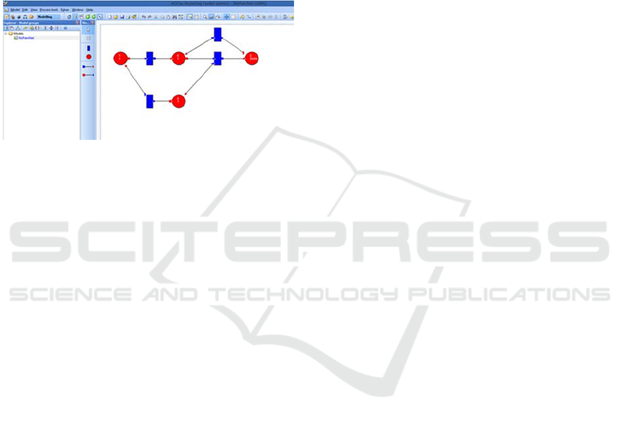
The Petri Net metamodel was implemented in
MM-DSL then translated and executed in ADOxx
(Karagiannis and Mayr and Mylopoulos, 2016). In
Figure 6. we can see a screen capture from the Petri
Net modeling tool in which we built the graphic
model in example 1 (Figure 5) that we executed and
it works.
Figure 6: Screen capture from the PN modeling tool.
6 CONCLUSIONS
The sketch L
0
represents the meta-metamodel, i.e. it
is the basic sketch of the meta-metamodel.
Any functor H
1
:L
0
Set represents the basic
sketch of a metamodel, i.e. the basic sketch of a
Modeling Method that we have denoted with L
1
. The
set of models H
, k0 together with the natural
transformations between models form a category that
we call the Modeling Method Category. Each object
in this category is a Modeling Method.
Each functor H
2
:L
1
Set is a model that can be
specified within this Modeling Method.
The set of models H
, k0 together with the
natural transformations between models form a
category that we call the category of specifiable
models in a Modeling Method. Each object in this
category is a specifiable model in a Modeling
Method, represented by the sketch L
1
.
In the category theory, models are functors that
map the sketches into the Set category that leads to a
lot of important features on simulation, analysis, and
process improvement.
Universal constructs in category theory are the
basis for implementing a package of mechanisms and
algorithms in a modeling method. In fact, the
categories theory constructs, provide us with a
package of universally valid results that could be
implemented in modeling method and which would
be valid in any model built according to category
theory.
Based on these functors, important issues such as
model migration and model equivalence can be
solved. The difficult problem of Database Migration
can also be solved.
The paths from the CIT category represent, in fact,
the admissible execution rules on which real-time
deviations can be reported to be corrected.
The CIT category arrows that represent natural
transformations are objects that can have attributes
that dynamically sustain a series of data such as the
trace of the process, the frequency of execution of the
activities, the estimated time, the estimated cost, the
probability that an activity will be executed by a
certain resource, etc.
Also, on the basis of some information from the
CIT category, it is possible to give indications to the
activities to be executed and make recommendations
on the most favorable route based on criteria such as
minimizing the cost, minimizing the time until the
case completion, etc.
REFERENCES
Dimitris Karagiannis, H. Kühn, 2002. Metamodelling
Platforms. Invited paper in: Bauknecht, K.; Tjoa, A
Min.; Quirchmayer, G. (eds.): Proceedings of the Third
International Conference EC- Web 2002 - Dexa 2002,
Aix-en-Provence, France, September 2-6, 2002, LNCS
2455, Springer-Verlag, Berlin, Heidelberg.
Dimitris Karagiannis, N. Visic, 2011. Next Generation of
Modelling Platforms. Perspectives in Business
Informatics Research 10th International Conference,
BIR 2011 Riga, Latvia, October 6-8, 2011 Proceedings.
Dimitris Karagiannis, Heinrich C. Mayr, John Mylopoulos,
2016. Domain-Specific Conceptual Modeling
Concepts, Methods and Tools. Springer International
Publishing Switzerland 2016.
Dimitris Karagiannis, Junginger S., Strobl R., 1996.
Introduction to Business Process Management Systems
Concepts. In: Scholz-Reiter B., Stickel E. (eds)
Business Process Modelling. Springer, Berlin,
Heidelberg, 1996
Ernest G. Manes, Michael A. Arbib, 1986. Algebraic
Approaches to program semantics, Springer Verlag
New York Berlin Heidelberg London Paris Tokyo –
1986
Michael Barr, Charles Wells, 2012. Category Theory For
Computing Science, Reprints in Theory and
Applications of Categories, No. 22, 2012.
Michael Barr, Charles Wells, 2002. Toposes, Triples and
Theories, November 2002.
R. F. C. Walters, 2006. Categories and Computer Science,
Cambridge Texts in Computer Science, Edited by D. J.
Cooke, Loughborough University, 2006.
MODELSWARD 2019 - 7th International Conference on Model-Driven Engineering and Software Development
288

Mathias Weske, 2012. Business Process Management -
Concepts, Languages, Architectures, 2nd Edition.
Springer 2012, ISBN 978-3-642-28615-5, pp. I-XV, 1-
403.
Winskel Glynn, 2009. Topics in Concurrency, Lecture
Notes, April 2009.
Wil M.P. van der Aalst, 2011. Process Mining Discovery,
Conformance and Enhancement of Business Processes,
Springer-Verlag Berlin Heidelberg 2011.
W.M.P. van der Aalst and K.M. van Hee, 2004. Workflow
Management: Models, Methods, and Systems. MIT
press, Cambridge, MA, 2004.
Categorical Modeling Method, Proof of Concept for the Petri Net Language
289
