Deep Reinforcement Learning for Pellet Eating in Agar.io
Nil Stolt Ans
´
o
1
, Anton O. Wiehe
1
, Madalina M. Drugan
2
and Marco A. Wiering
1
1
Bernoulli Institute, Department of Artificial Intelligence, University of Groningen, Nijenborgh 9, Groningen, Netherlands
2
ITLearns.Online, Utrecht, Netherlands
Keywords:
Deep Reinforcement Learning, Computer Games, State Representation, Artificial Neural Networks.
Abstract:
The online game Agar.io has become massively popular on the internet due to its intuitive game design and its
ability to instantly match players with others around the world. The game has a continuous input and action
space and allows diverse agents with complex strategies to compete against each other. In this paper we focus
on the pellet eating task in the game, in which an agent has to learn to optimize its navigation strategy to grow
maximally in size within a specific time period. This work first investigates how different state representa-
tions affect the learning process of a Q-learning algorithm combined with artificial neural networks which are
used for representing the Q-function. The representations examined range from raw pixel values to extracted
handcrafted feature vision grids. Secondly, the effects of using different resolutions for the representations
are examined. Finally, we compare the performance of different value function network architectures. The
architectures examined are two convolutional Deep Q-networks (DQN) of varying depth and one multilayer
perceptron. The results show that the use of handcrafted feature vision grids significantly outperforms the
direct use of raw pixel input. Furthermore, lower resolutions of 42× 42 lead to better performances than larger
resolutions of 84 × 84.
1 INTRODUCTION
Reinforcement learning (RL) is a machine learning
paradigm that uses a reward function that assigns a
value to a specific state an agent is in as a supervi-
sion signal (Sutton and Barto, 2017). The agent at-
tempts to learn what actions to take in an environment
to maximize this reward signal. The environment for
this research is based on the game of Agar.io, which
is itself inspired by the behaviour of biological cells.
The player controls circular cells in a 2D plane (as
if laid out on a Petri dish) which follow the player’s
mouse cursor. The player can signal their cells to split
or eject little vesicles of mass. Cells of a player can
eat small food pellets scattered in the environment or
other smaller enemy player-controlled cells to grow in
size. The environment of Agar.io is therefore very in-
teresting for RL research, as it is mainly formed by the
behavior of other (larger) players on the same plane, it
is stochastic and constantly changing. Also the output
space is continuous, as the cells of the player move to-
wards the exact position of the mouse cursor. On top
of that, the complexity of the game can be scaled by
introducing or removing additional features. This pa-
per therefore studies how to use RL to build an intelli-
gent agent for this game, especially focusing on how
to represent the game state for the agent.
The use of artificial neural networks (ANN) has
demonstrated great promise at learning representa-
tions of complex environments. Tesauro was among
the first to show that near-optimal decision mak-
ing could be learned in the large state space of the
game Backgammon through the use of a multilayer
perceptron (MLP) and temporal difference learning
(Tesauro, 1995). Over the years, this principle has
been extended through the use of convolutional neu-
ral networks (CNNs). This has been shown to achieve
human level performance by learning from solely
pixel values in a variety of Atari games (Mnih et al.,
2013), and even first-person perspective 3D games
like Doom (Lample and Chaplot, 2017).
A problem of directly learning from pixel values is
that the state spaces are extremely large, which results
in large computational requirements. One approach to
overcoming the issue of large state spaces is by pre-
processing the game state in order to extract features
that boost performance and reduce the amount of po-
tentially irrelevant information required for the net-
work to process. The use of vision grids is one such
approach that has been employed in games such as
Ansó, N., Wiehe, A., Drugan, M. and Wiering, M.
Deep Reinforcement Learning for Pellet Eating in Agar.io.
DOI: 10.5220/0007360901230133
In Proceedings of the 11th International Conference on Agents and Artificial Intelligence (ICAART 2019), pages 123-133
ISBN: 978-989-758-350-6
Copyright
c
 2019 by SCITEPRESS – Science and Technology Publications, Lda. All rights reserved
123

Starcraft (Shantia. et al., 2011) and Tron (Knegt et al.,
2018) by extracting hand-crafted features into grids.
Such methods can greatly simplify the state space and
allow for a decreased network complexity. Despite
this benefit, feature extraction might introduce biases
and has no guarantee to achieve the same performance
as a network being fed the raw game representation
(given enough training time).
A widely successful algorithm for reinforcement
learning that acts on state representations is Q-
Learning (Watkins, 1989). This algorithm can be
combined with a function approximator to estimate
the Quality, or long-term reward prospect, of a state-
action pair. This algorithm has been used in the re-
search mentioned above on Atari games (Mnih et al.,
2015), Doom (Lample and Chaplot, 2017), and Tron
(Knegt et al., 2018). In Atari games, Doom and Tron,
the possible actions in each state are equivalent to the
buttons that the player can press. In Agar.io, the rela-
tive position of the mouse cursor on the screen is used
to direct the player. This has a range of continuous
values, similarly to real-life robotic actuators, which
are therefore discretized in this work.
Contributions of this Paper. This paper explores
how the complexity of the state space affects the con-
vergence and final performance of the reinforcement
learning algorithm. This is explored through a core
task of the game: pellet collection. In this task, the
agent has to navigate in the environment and eat as
many food pellets as possible.
More specifically, this research focuses on how
different state representations, varying resolutions of
such state representations, and varying the structure
of the function approximators affect the performance
of the Q-learning algorithm. First, different kinds of
low-level information used in the state representation
are compared, each one providing a different kind
of information. This includes grayscale pixel values,
RGB pixel values, and a semantic vision grid for pel-
lets in the environment. The effect of the resolution
of these state representations is also explored. Finally
the ability of Q-learning to achieve a good playing
performance is examined when using two different
CNN structures (which differ in the number of layers)
which are also compared to the use of an MLP.
Paper Outline. Section 2 outlines the fundamental
principles behind Q-learning combined with ANNs
and the techniques used to enhance its performance.
In Section 3, the game of Agar.io and the different
state representations are described. The experimen-
tal setup follows in Section 4, where the network
structures and other experimental parameters are de-
scribed. Next, Section 5 shows and discusses the ex-
perimental results. Section 6 gives the conclusions.
2 REINFORCEMENT LEARNING
This paper follows the general conventions (Sutton
and Barto, 2017) to model the reinforcement learning
(RL) problem as a Markov decision process (MDP).
In a Markov Decision Process an agent can take an
action in a state to get to a new state, for which it re-
ceives a scalar reward. The transition from the state
to the new state has the Markov property: the stochas-
tic transition probabilities between the states are only
dependent on the current state and selected action.
To model the RL problem as an MDP, it must be
defined what a state constitutes of. In short, the state
consists of the properties the environment has and
how the agent perceives the available relevant infor-
mation. The transition between a state and an action
to a new state is handled by the game engine.
2.1 The Reward Function
In RL there must be some function that maps a state
transition to a reward, also called the reward function.
The aim of the agent in RL is to maximize the total
expected reward that the agent receives in the long
run through this reward function, also called the gain
(G):
G =
∞
∑
t=0
r
t
· γ
t
(1)
r
t
indicates the reward the agent receives at time t and
γ indicates the discount factor. This discount factor is
a number between 0 and 1 and controls how much fu-
ture rewards are discounted and therefore how much
immediate rewards are preferred.
2.2 Q-Learning
Q-learning (Watkins, 1989) predicts the quality (Q-
value) of an action in a specific state. By iterating
through all possible actions in a state, the algorithm
picks the action with the highest Q-value as the ac-
tion that the agent should take in that state. The Q-
value indicates how much reward in the long term, or
how much gain, the agent can expect to receive when
choosing action a in state s. This prediction is up-
dated over time by shifting it towards the reward that
the agent got for taking that action and the predicted
value of the best possible action in the next state.
As Q-learning iterates over all possible actions in
a state, the action space cannot be continuous. There-
fore we discretize the action space by laying a grid of
actions over the screen (Figure 1). Every center point
of a square in the grid indicates a possible mouse po-
sition that the algorithm can choose.
ICAART 2019 - 11th International Conference on Agents and Artificial Intelligence
124

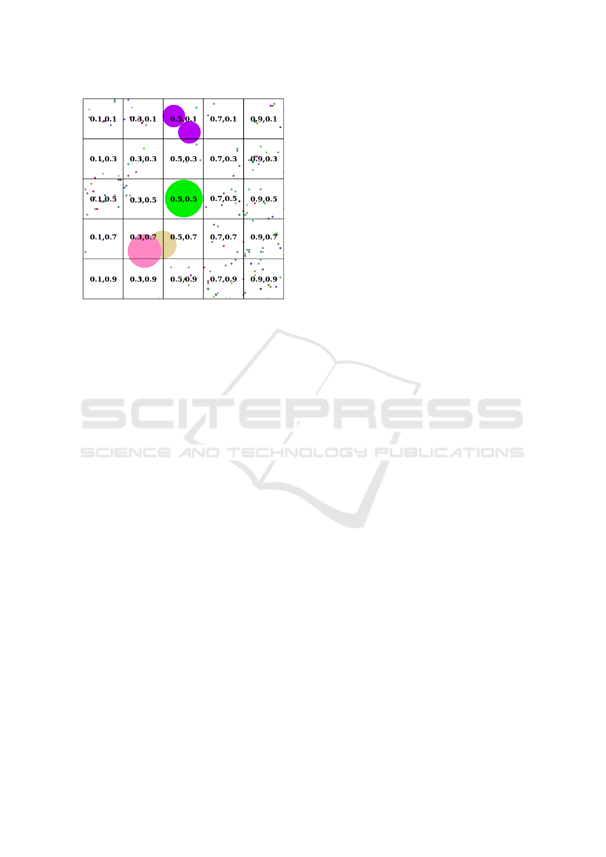
Figure 1: Possible action coordinates are laid out in a grid-
like fashion. At a given state, the network chooses the
square with the highest Q-value as an action. In total, there
are 25 possible actions.
To predict the Q-value for an action in a state,
an artificial neural network (ANN) is used, which is
trained through backpropagation. To construct the
ANN to predict the Q-values we took inspiration from
the network structure proposed in (Mnih et al., 2013).
This architecture feeds the state as an input to the net-
work and has one output node per possible action.
The tabular Q-learning update for a transition from
state s
t
after selecting action a
t
with reward r
t
and the
new state s
t+1
is:
Q(s
t
, a
t
) = Q(s
t
, a
t
) · (1 − α) + α · (r
t
+ γ · max
a
Q(s
t+1
, a))
In this formula α indicates the learning rate. This
formula is adapted so that it can be used to train an
ANN by calculating the target for backpropagation
for a specific state-action pair (s
t
, a
t
):
Target(s
t
, a
t
) = r
t
+ γ · max
a
Q(s
t+1
, a) (2)
2.2.1 Exploration
It is necessary to explore the action space throughout
training to avoid being stuck in local optima. For Q-
learning the ε-greedy exploration (Sutton and Barto,
2017) was chosen due to its simplicity. The ε value
indicates how likely it is that a random action is cho-
sen, instead of choosing greedily the action with the
highest Q-value. For this research the ε value is an-
nealed exponentially from 1 to a specific value close
to 0 over the course of training. The ε value should de-
crease over time, as this allows the agent to progress
more in the game by taking more greedy actions. This
causes the agent to progress steadily while exploring
alternative actions over the course of training.
2.2.2 Target Networks
To stabilize Q-learning when combined with artificial
neural networks, (Mnih et al., 2013) introduced target
networks. As Q-learning computes targets by max-
imizing over the possible actions taken in the next
state, the combination of this algorithm with function
approximators can lead to the deadly triad (Sutton and
Barto, 2017). This deadly triad gives a high probabil-
ity of the Q-function to diverge from the true func-
tion over the course of training. A possible remedy
to this problem is Double-Q-learning (Hasselt, 2010),
which uses two Q-value networks. For the training
of one network, the other network is used to calcu-
late the Q-value of the action in the next state of a
transition to avoid the positive feedback loop of the
deadly triad. Mnih et al. simplify this approach by in-
troducing a target network in addition to the Q-value
network. The parameters of the Q-value network are
copied to the target network every time after a cer-
tain amount of steps. This requires no need to train
a new separate network, but the maximization of the
Q-values is still done by a slightly different network,
therefore mitigating the unwanted effect.
2.2.3 Prioritized Experience Replay
Lin introduced a technique named experience re-
play to improve the performance of Q-learning (Lin,
1992). The technique has been shown to work well
for DQN (Mnih et al., 2015). When using experience
replay every transition tuple (s
t
, a
t
, r
t
, s
t+1
) is stored
in a buffer instead of being trained on directly. If this
buffer reaches its maximum capacity the oldest tran-
sitions in it get replaced. To train the value network
using experience replay in every training step N ran-
dom transitions (experiences) from the replay buffer
are sampled with replacement to create a mini-batch.
For each of the transitions in the mini-batch the target
for s
t
and a
t
is calculated and then the value network
is trained on this mini-batch.
This form of experience replay offers a big ad-
vantage over pure online Q-learning. One assump-
tion of using backpropagation to train an ANN is that
the samples that are used to train in the mini-batches
are independent and identically distributed. This as-
sumption does not hold for online Q-learning, as each
new transition is correlated with the previous transi-
tion. Therefore random sampling from a large buffer
Deep Reinforcement Learning for Pellet Eating in Agar.io
125

of transitions partially restores the validity of this as-
sumption. Furthermore, with experience replay, expe-
riences are used much more effectively, as the agent
can learn multiple times from them.
As an enhancement of experience replay, prior-
itized experience replay (PER) has been introduced
(Schaul et al., 2015). PER does not sample uniformly
from the replay buffer, but instead assigns the sam-
pling probability to an experience i:
P(i) =
T DE
α
i
∑
k
T DE
α
k
(3)
Here, the α coefficient determines how much pri-
oritization is used, α = 1 would mean full prioritiza-
tion. TDE stands for the temporal difference error of
transition i, computed as:
T DE
i
= r
t
+ γ · max
a
Q(s
t+1
, a) − Q(s
t
, a
t
) (4)
This implies that the badly predicted transitions
are replayed more often in the network, which was
shown to lead to faster learning and better final per-
formance (Schaul et al., 2015).
More transitions with high TDEs trained on in
PER leads to proportionally larger changes in the
weights of the network. Schaul et al. introduced
an importance sampling weight which decreases the
magnitude of the weight change in the MLP for tran-
sition i anti-proportionally to its T DE
i
. This is done
to reduce the bias of training on average on more high
TDE transitions. Therefore, a weight w
i
is applied
to the weight changes induced by each transition i of
magnitude:
w
i
= (
1
N
·
1
T DE
i
)
β
(5)
In this formula N is the batch size and β controls the
amount of applied importance sampling. In practice
the weights are used in the Q-learning update by mul-
tiplying the prediction error for transition i, used in
backpropagation, by w
i
.
3 THE GAME AND STATE
REPRESENTATION
Agar.io is a multi-player online game in which the
player controls one or more cells. The game has a
top-down perspective on the map of which the size of
the visible area of the player is based on the mass and
count of their cells. The goal of the game is to grow a
player as much as possible by absorbing food pellets,
viruses, or other smaller enemy player’s cells. The
game itself has no end. Players can join an ongoing
game at any point in time. Players start the game as a
single small cell in an environment with other player’s
cells of all sizes. When all the cells of a player are
eaten, that player loses and may choose to re-enter
the game.
In every time step, every cell in the game loses a
small percentage of its mass. This makes it harder for
large cells to grow quickly and it punishes inaction or
hesitation. The game has simple controls. The cur-
sor’s position on the screen determines the direction
all of the player’s cells move towards. The player also
has the option to ’split’, in which case every player
cell (given the cell has enough mass) splits into two
cells of the same mass, both with half the mass of the
original cells. Furthermore, the player has an option
to have every cell ’eject’ a small mass blob, which is
eaten by other cells or viruses. Although, the game
has relatively simple core mechanics, the game also
has a complex and dynamic range of environments.
The larger a cell is, the slower it moves. This forces
players to employ strategies with long-term risks and
rewards.
For the purpose of this research, the game was
simplified to fit the computational resources available.
The used version of the game has disabled viruses
and runs with only one player. Furthermore, eject-
ing and splitting actions were disabled for the exper-
iments in this paper. Ejecting is only useful for very
advanced strategies, and splitting requires tracking of
when the player’s cells are able to merge back to-
gether over long time intervals. The use of these ac-
tions would require recurrent neural networks such as
LSTMs (Hochreiter and Schmidhuber, 1997) which
are outside of the scope of this research. Figure 2
shows a screenshot of the developed clone of Agar.io
used for this research.
We also introduce a ’Greedy’ bot to the game
to compare against the RL agents. This bot is pre-
programmed to move towards the cell with the high-
est cell mass to distance ratio. The bot ignores cells
with a mass above its biggest own cell’s absorption
threshold. The bot also has no splitting or ejecting
behavior. This relatively naive heuristic, outperforms
human players at early stages of the game. On the
other hand, the heuristic is often outperformed later
in the game by abusing its lack of path planning and
general world knowledge.
The aim in Agar.io is to grow as big as possible.
That means the agent has the aim to maximize the
mass of its cell in the shortest amount of time pos-
sible. This leads to the idea of the reward being the
change in mass (m) between the previous state and
the current state:
r
t
=
(
0, if t = 0
m
t
− m
t−1
, otherwise
(6)
ICAART 2019 - 11th International Conference on Agents and Artificial Intelligence
126

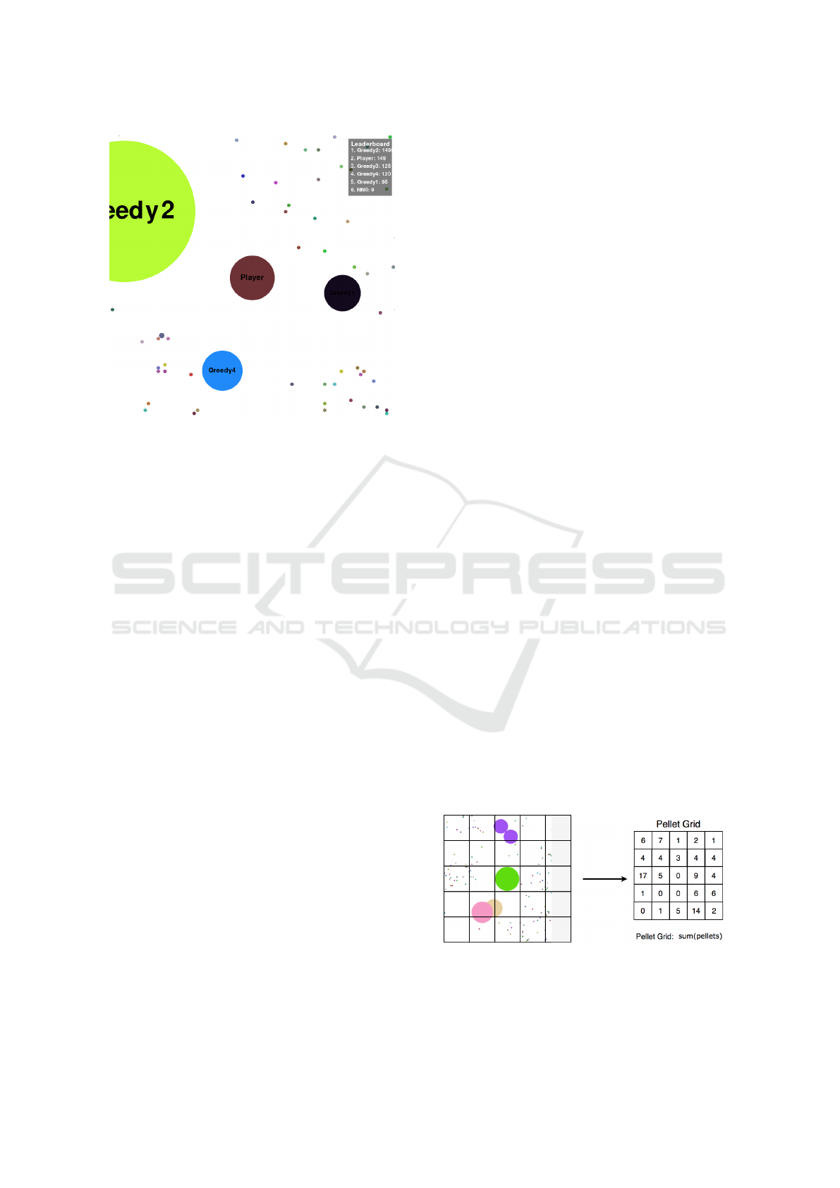
Figure 2: A clone of the game Agar.io used for this research.
The player has one cell in the center of the screen. This
player is in danger of being eaten by the Greedy bot seen on
the top left, the other cells have a similar size as the player’s
cell and therefore pose no danger. The little colored dots are
pellets that can be consumed to grow in mass.
This research applies frame-skipping to the MDP.
In frame skipping a certain number of frames, or
states, are skipped and the action that the agent chose
is applied during all of these skipped frames. Also the
rewards during these skipped frames are summed up
until the next non-skipped state where the sum total
is used as the reward. Frame skipping offers a direct
computational advantage, as it allows the agent to not
have to calculate the best action in every single frame
of the game. More importantly, frame skipping leads
to successive states in the MDP to be more differ-
ent from each other than without frame skipping and
leads to higher rewards, simply because more steps
happened in between states. Making successive states
more different from each other makes it easier for a
function approximator to differentiate states. Larger
and more different rewards also have a positive effect
on the training speed.
3.1 The State Representation
The information used in state representations can
have varying levels of abstraction. The choice of a
given state representation often brings positive and
negative influences on the algorithm’s learning pro-
cess, which the designer has to balance optimally.
State representations with high levels of abstraction
usually have the environment information prepro-
cessed before it is fed to the algorithm. This has the
advantage of allowing for a simpler network which
takes less training time to converge. However, state
representations of hand-crafted features are inherently
biased due to being created with the programmer’s
own heuristic in mind. An example of this is Bom
et al.’s paper on learning to play Ms. Pac-Man (Bom
et al., 2013), where a small neural network learns to
play the game by using a representation that includes
the distance to the closest collectable pills as deter-
mined by an A* search algorithm.
On the other end of the spectrum there are ap-
proaches where the unfiltered raw data of the envi-
ronment is fed to the learning algorithm. The sim-
plicity of this approach allows for agents to learn in
complex state-action spaces for which humans might
have non-optimal existing heuristics. The downside is
that the large number of parameters the networks are
required to have, brings issues with processing power
and amount of training time before convergence.
One of the aims of this paper is to research how
state representations of the same resolution, but with
varying levels of preprocessing compare to one an-
other. The base representation of the game is the raw
state representation of the game, which comes in the
form of RGB pixel values. The second state repre-
sentation uses the grayscale pixel values. A player
in Agar.io aims to locate food pellets and cells in
its view against a white background. Processing the
RGB channels into a single grayscale channel reduces
the amount of weight tuning required for the network
in order to extract non-white objects. This process-
ing is performed by a pixel-wise averaging across the
RGB channels. The third state representation is a se-
mantic representation of objects in the environment.
This consists of a vision grid in which every individ-
ual area unit has a value equal to the amount of food
pellets contained in that area (see Figure 3). For the
following experiments, the grid values at given areas
were obtained from the game engine itself to reduce
computational costs, but one could theoretically ob-
tain these values from the RGB pixel values of the
real game using preprocessing techniques.
Figure 3: The semantic state representation consists of a
vision grid laid out on the player’s view. Values are then
extracted from each area unit based on how many food pel-
lets are present in it. Note that in the pellet eating task, the
learning agent is the only player in the game.
Deep Reinforcement Learning for Pellet Eating in Agar.io
127

Another aim of this paper is to explore how much
the performance is influenced by the resolution of
these representations. The DQN approach has shown
success with state representation sizes of 84 by 84
(Mnih et al., 2015), but one could hypothesize that as
the representation resolution drops, it will be harder
for the network to understand the specific situation of
the game. Given this, semantic representations should
be expected to perform marginally better than pixel
values at lower resolutions.
The last aim of this paper is to compare how dif-
ferent representations perform with different architec-
tures. Every subsequent layer in a neural network can
be thought of as providing recognition of more ab-
stract concepts. Providing the network with a more
semantically complex state representation to begin
with, might relieve the network from the need to ex-
tract objects such as circles (for pellets), as well as
features such as the size of the circles (for estimating
the mass of the cell). This hypothesis will be tested by
comparing the performance of the pixel and semantic
representations between a CNN with 3 convolutional
layers to that of a CNN with 2 convolutional layers.
The first network has the same structure as the one
used in the 2015 DQN paper (Mnih et al., 2015). With
the only difference being that the one used here only
uses one single channel for the current representation
of the game, whereas the one used by Mnih et al. use
convolution over the 4 last frames. The second ex-
amined CNN has a similar structure to the 2013 DQN
paper (Mnih et al., 2013).
Furthermore, to emphasize how the semantic rep-
resentation is used to achieve high performances with
relatively small networks, the mentioned methods
will also be compared to that of a standard MLP with-
out convolutional layers that uses a semantic state rep-
resentation of resolution 11 by 11.
4 EXPERIMENTAL SETUP
This research uses the OpenAI baselines repository
(Dhariwal et al., 2017) for prioritized experience re-
play to enhance reproducibility. The hyperparameters
have been tuned using a coarse search through param-
eter space and can be found in the appendix.
4.1 General Experimental Setup
In all experiments, the environment resets after
20,000 game steps. This is considered to be one
episode. Upon reset the agent is reassigned a new cell
with mass 10 at a random location and all pellet loca-
tions are randomized. This is done to avoid that the
learning agent learns peculiarities of pellet locations
on the map and to force the agent to also learn to deal
with low cell mass strategies. Furthermore, to avoid
the network from overfitting to one particular color
in the pixel value representations, we also have the
player cell color randomized every time an episode
ends. Pellet colors are always randomized when new
pellets are generated in the game.
Each algorithm instance was trained with 300,000
state transitions. Given the network used a frame
skip rate of 10, one state transition experience was
generated every 11 in-game frames, giving a total
of 3,300,000 game steps. These states were gener-
ated on-line as the network learned to play and stored
into the experience replay buffer of size 20,000. Ev-
ery training step, the network was trained on 32 ex-
periences sampled (with replacement) from a single
batch. On an Intel Xeon E5 2680v3 CPU @2.5Ghz it
took between 32 to 84 hours to train each individual
CNN run depending on the trial. State representations
of 42 by 42 in resolution were at the lower end due
to their smaller amount of network parameters, while
resolutions of 84 by 84 took the longest to train on.
On the other hand, the MLP runs took approximately
5.5 hours.
Every 5% of the training process the performance
of one agent is tested five times. The noise factor of
the agent (ε of ε-greedy) is then set to zero. In this
environment the agent collects pellets for 15,000 in-
game steps. Furthermore, after training is completed
the agent is placed in the environment 10 times to
measure the final performance.
A simulation refers to the complete training and
testing process as described before. The perfor-
mances for each experimental condition are calcu-
lated by taking the mean scores from 10 independent
simulations.
4.2 Network Structures
The simple MLP architecture consists of a variable
input length, 3 fully connected layers, and an output
layer. All artificial neural networks were constructed
using Keras 2.1.4 (Chollet et al., 2015). The input to
the MLP consists of the grid of the semantic repre-
sentation, which was first flattened into a 1D vector,
and then had 2 extra values appended to it: the cur-
rent mass of the player, and the ’field of view’ (FoV)
size of the player. These two extra values are infor-
mation the human player has implicit access to in the
real game through estimation of the total mass and
FoV size by comparison to features such as the rel-
ative sizes of a food pellet, or the game background.
This source of information is useful, as the optimal
ICAART 2019 - 11th International Conference on Agents and Artificial Intelligence
128

strategy in the game changes depending on size. For a
state’s semantic representation resolution of 11 by 11
where a pellet vision grid is used, the 1D input vector
of the network would be 123 in length. This input is
then fed into 3 subsequent fully connected layers of
250 rectified linear units each. This is then followed
by an output layer of 25 linear units which refer to the
25 possible actions. The output layer, as specified in
the ’Reinforcement Learning’ section, has units sym-
bolizing the Q-value of a possible mouse position on
the screen using a grid-like fashion (see Figure 1).
The first CNN architecture has the same structure
as that used for Atari games in the 2015 DQN paper
(Mnih et al., 2015), with the difference being that the
structures used here only use the current frame in the
input for the convolution. The default input consists
of 84 by 84 units in length, the number of channels
is dependent on the type of representation used. The
first convolutional layer uses a kernel size of 8 by 8
with stride 4 for a total of 32 filters. The second con-
volutional layer uses a kernel size of 4 by 4 with stride
2 for 64 filters. The third convolutional layer uses
a kernel size of 3 with stride 1 for 64 filters. Every
convolutional layer applies a rectified linear activa-
tion function. At this point in the network, the current
layer’s output was flattened and, similar to the case of
the MLP’s input, the values for the mass of the player
and the FoV size were appended to it. Next, this 1D
vector was fed to a fully connected layer of 512 recti-
fier units, which was then followed by an output layer
of 25 linear units.
Lastly, the second CNN architecture has a similar
structure to the first one, but has only 2 convolutional
layers. Again, the input by default consists of 84 by
84 units in length. The number of channels is depen-
dent on the type of representation used. The first con-
volutional layer uses a kernel size of 8 by 8 with stride
4 and a total of 32 filters. The second convolutional
layer uses a kernel size of 4 by 4 with stride 2 and
64 filters. Every convolutional layer applies a recti-
fied linear activation function. Just like in the other
CNN architecture, at this point the layer’s output is
flattened into a 1D array and gets appended the mass
and FoV player values. Next, a fully connected layer
of 256 rectifier units is used, which is then followed
by an output layer of 25 linear units.
5 EXPERIMENTAL RESULTS
5.1 General Results
Figure 4 shows the test results with different reso-
lutions for the vision grid representation using both
CNN architectures. The 42 by 42 resolutions per-
form better than every other resolution. The 84 by
84 resolution performs the second best closely fol-
lowed by the 63 by 63 resolution. Unsurprisingly, as
seen in Figure 5, the 42 by 42 resolution also achieves
good training performances the fastest due to its lower
number of trainable parameters. The 3 convolutional
layer network seems to also achieve slightly better
performances than the 2 convolutional layer CNN for
resolutions of 42 by 42 and 63 by 63, but not for 84
by 84. The MLP architecture with the 11 by 11 res-
olution seems to achieve a higher performance than
both CNNs using 84 by 84 resolutions, although not
as high as CNNs using 42 by 42 resolutions. The
MLP seems to learn at a similar rate as 84 by 84 CNN
resolutions (see Figure 5).
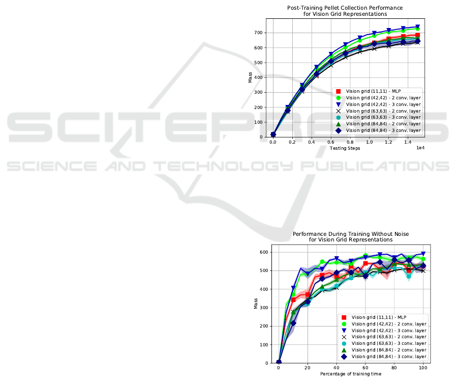
Figure 4: Post-training performance of vision grid represen-
tations with differing resolutions for the two CNN architec-
tures, as well as for the MLP architecture with a 11 by 11
resolution. Each point represents the average of the 10 test-
ing rounds and the shaded area denotes its 1 standard error
(SE) range. Results are averages of 10 simulations.
Figure 5: During-training performance of vision grid rep-
resentations with differing resolutions for the two CNN ar-
chitectures, as well as for the MLP architecture with a 11
by 11 resolution. Each point represents the average of the 5
testing rounds and the shaded area denotes its 1 SE range.
Deep Reinforcement Learning for Pellet Eating in Agar.io
129

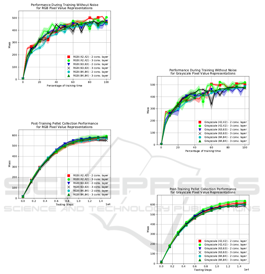
Figure 6: During-training performance of RGB pixel value
representations with differing resolutions for the two CNN
architectures. Each point represents the average of the 5
testing rounds and the shaded area denotes its 1 SE range.
Figure 7: Post-training performance of RGB pixel value
representations with differing resolutions for the two CNN
architectures. Each point represents the average of the 10
testing rounds and the shaded area denotes its 1 SE range.
The RGB pixel value representations seem to all
have similar during-training performances as seen in
Figure 6, suggesting that resolution does not have
much of an effect on the learning process of the net-
works for the resolutions tested with RGB pixel val-
ues. This is further emphasized by Figure 7, where
there are no noticeable differences between the reso-
lutions or architectures in post-training performance.
Lastly, the grayscale pixel value representation ap-
pears to have trends similar to those of vision grids,
but not to the same extent. The during training perfor-
mance of the 42 by 42 resolutions seems to converge
at a slightly higher performance than the other 2 reso-
lutions (see Figure 8). The post-training performance
seen in Figure 9 also seems to indicate that 42 by 42
resolutions have a higher performance after 300,000
training steps.
In order to observe how different kinds of state
representations compare to one another, some of the
highest performing runs were plotted together as seen
in Figures 10 and 11. The best results are obtained
with the vision grids with resolution 42 × 42. The 42
by 42 grayscale representation on a 2 convolutional
layer network seems to achieve a similar final perfor-
mance as both 84 by 84 vision grid representations.
This grayscale run is noticeably better than the plotted
42 by 42 RGB representation with a 3 convolutional
layer network in terms of final performance.
Figure 8: During-training performance of grayscale pixel
value representations with differing resolutions for the two
CNN architectures. Each point represents the average of the
5 testing rounds and the shaded area denotes its 1 SE range.
Figure 9: Post-training performance of grayscale pixel
value representations with differing resolutions for the two
CNN architectures. Each point represents the average of
the 10 testing rounds and the shaded area denotes its 1 SE
range.
The post-training performances for all conditions
are listed in Table 1. The column ’Mean Performance’
shows the mean testing scores across all 10 tests of
all 10 simulations. The column ’Mean Max Perfor-
mance’ shows the average maximum scores across all
10 tests of all 10 simulations. The top scoring con-
dition appears to be ’Vision grid (42,42) - 3 conv.
layers’ with a max score of 763. Comparing its max
score to its 2 convolutional layer counterpart (which
ICAART 2019 - 11th International Conference on Agents and Artificial Intelligence
130

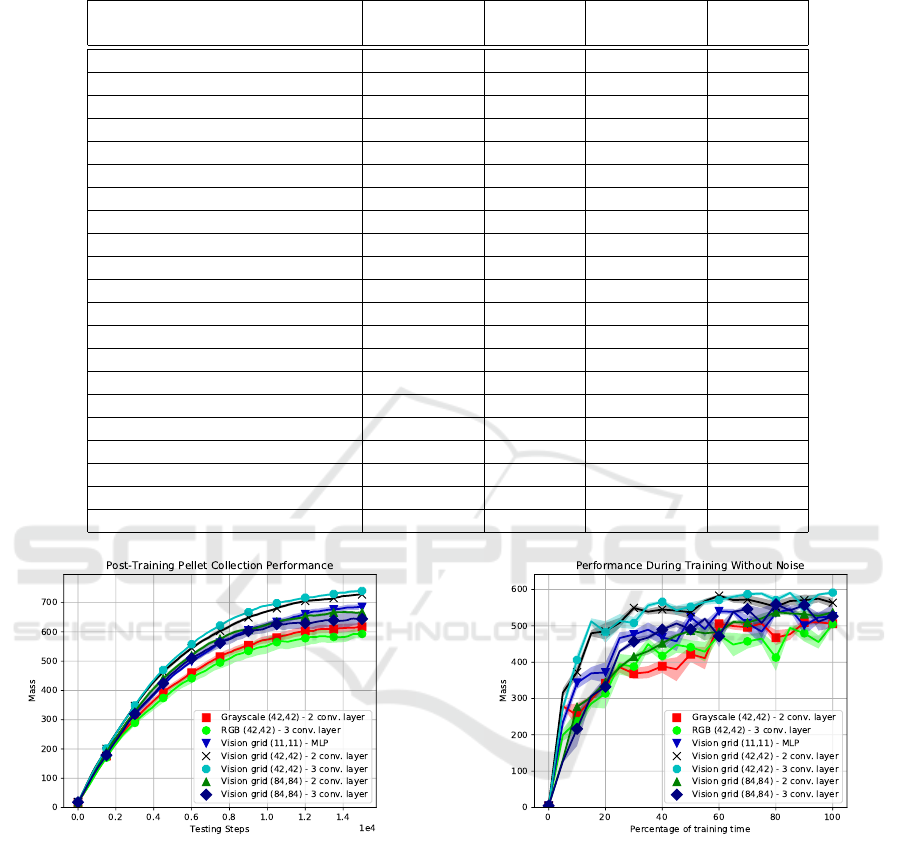
Table 1: Post-training mean performances across 10 simulations. The ’Mean Performance’ column contains the mean mass
value for the post-training averaged performance curve. The ’Mean Max Performance’ column shows the max scores of the
post-training averaged performance curve.
Mean Std. Error Mean Max Std. Error
Performance Mean Performance Max
Random 18 0.1 31 0.2
Greedy Heuristic 527 0.3 693 0.6
Vision grid (11,11) MLP 481 2.8 704 5.9
Vision grid (42,42) 3 conv. layer 537 0.6 763 0.9
Vision grid (42,42) 2 conv. layer 526 1.1 750 1.1
Vision grid (63,63) 3 conv. layer 479 1.3 688 0.6
Vision grid (63,63) 2 conv. layer 461 1.4 662 1.8
Vision grid (84,84) 3 conv. layer 480 5.7 675 5.4
Vision grid (84,84) 2 conv. layer 494 1.2 696 1.1
Grayscale (42,42) 3 conv. layer 471 4.2 669 4.9
Grayscale (42,42) 2 conv. layer 449 4.5 648 6.8
Grayscale (63,63) 3 conv. layer 446 2.0 617 1.2
Grayscale (63,63) 2 conv. layer 448 3.1 625 1.1
Grayscale (84,84) 3 conv. layer 442 2.1 632 1.7
Grayscale (84,84) 2 conv. layer 439 1.5 627 2.2
RGB (42,42) 3 conv. layer 432 7.2 628 6.8
RGB (42,42) 2 conv. layer 425 7.0 609 9.9
RGB (63,63) 3 conv. layer 421 7.8 588 7.4
RGB (63,63) 2 conv. layer 436 2.3 609 2.7
RGB (84,84) 3 conv. layer 421 7.8 588 7.4
RGB (84,84) 2 conv. layer 427 0.9 598 1.6
Figure 10: Post-training performance of various top-
performing runs of various representations and network ar-
chitectures. Each point represents the average of the 10 test-
ing rounds and the shaded area denotes its 1 SE range.
holds the second highest score) through the use of
a t-test yields a p-value of 0.019, suggesting there
is a significant difference between their maximum
scores. This method also significantly outperforms
the Greedy bot and the vision grid with the MLP.
5.2 Discussion
As seen in Figures 10 and 11, the best performances
are achieved by the CNN networks using vision grid
Figure 11: During-training performance of various top-
performing runs of various representations and network ar-
chitectures. Each point represents the average of the 5 test-
ing rounds and the shaded area denotes its 1 SE range.
representations. Although the MLP network achieves
a surprising performance despite its requirement of
having a low resolution state representation, both
CNN architectures using the vision grid with a 42 by
42 resolution reach a higher performance at a faster
pace.
The performance increase in relation to the MLP
is likely due to the CNNs’ increased ability to pro-
cess local changes in the environment, thus not having
to evaluate potentially uncorrelated inputs far apart in
Deep Reinforcement Learning for Pellet Eating in Agar.io
131

the network’s input. This also allows a CNN to have
a higher resolution input while keeping its number
of parameters low, which helps explain why CNNs
reach higher performances faster than the MLP. The
deeper CNN architecture at 42 by 42 input resolution
has 118,969 trainable parameters while the MLP ar-
chitecture has 169,753.
The semantic representations yield a surprising
performance in comparison to the RGB and grayscale
pixel values. Even at resolutions of 11 by 11, the MLP
yields a significantly higher performance than using
RGB or grayscale pixel inputs. It should be noted
that the pixel value representations have not fully con-
verged after 300,000 training steps (see Figure 11),
and that it could be the case that given enough train-
ing time, these could match the performance of vision
grids. The same conclusion can be drawn for higher
vision grid resolutions (particularly 84 by 84), which
by the end of the training period have also not con-
verged.
A reason that could explain why the 63 by 63 reso-
lutions performed worse, is that the input dimensions
are odd-numbered while the kernel strides are even.
This causes the network to ignore 3 columns on the
right of the input and 3 columns on the bottom of the
input, leading to a loss of possibly important informa-
tion.
6 CONCLUSION
Deep reinforcement learning has obtained many suc-
cesses for optimizing the behavior of an agent with
pixel information as input. This paper focused on us-
ing deep reinforcement learning for the pellet collec-
tion task in the game Agar.io. We researched different
types of state representations and their influence on
the learning process of the Q-learning algorithm com-
bined with deep neural networks. Furthermore, dif-
ferent resolutions of these state representations have
been examined and combined with different artificial
neural network architectures.
The results show that the use of a vision grid
representation, which transforms raw pixel inputs to
a more meaningful representation, helps to improve
training speed and final performance of the deep Q-
network. Furthermore, a lower resolution (of 42× 42)
for both the vision grid representation and the raw
pixel inputs leads to higher performances. Finally,
the results show that a convolutional neural network
with 3 convolutional layers generally outperforms a
smaller CNN with 2 convolutional layers.
In future work, we aim to extend the algorithm so
that the agent learns to play the full game of Agar.io.
For this it would also be interesting to use the sam-
pled policy gradient (SPG) algorithm from (Wiehe
et al., 2018) and combine it with the used methods
from this paper. Finally, we want to compare the deep
Q-network approach from this paper to Deep Quality-
Value (DQV)-Learning (Sabatelli et al., 2018) for
learning to play the game Agar.io.
ACKNOWLEDGMENTS
We would like to thank the Center for Information
Technology of the University of Groningen for their
support and for providing access to the Peregrine high
performance computing cluster.
REFERENCES
Bom, L., Henken, R., and Wiering, M. A. (2013). Rein-
forcement learning to train Ms. Pac-Man using higher-
order action-relative inputs. In Adaptive Dynamic
Programming and Reinforcement Learning (ADPRL),
pages 156–163.
Chollet, F. et al. (2015). Keras.
Dhariwal, P., Hesse, C., Klimov, O., Nichol, A., Plappert,
M., Radford, A., Schulman, J., Sidor, S., and Wu, Y.
(2017). OpenAI baselines.
Hasselt, H. V. (2010). Double Q-learning. In Neural Infor-
mation Processing Systems (NIPS), pages 2613–2621.
Curran Associates, Inc.
Hochreiter, S. and Schmidhuber, J. (1997). Long Short-
Term Memory. Neural Computation, 9(8):1735–
1780.
Knegt, S. J. L., Drugan, M. M., and Wiering, M. A. (2018).
Opponent modelling in the game of Tron using re-
inforcement learning. In International Conference
on Agents and Artificial Intelligence (ICAART), pages
29–40. SciTePress.
Lample, G. and Chaplot, D. S. (2017). Playing FPS games
with deep reinforcement learning. In AAAI Confer-
ence on Artificial Intelligence, pages 2140–2146.
Lin, L.-J. (1992). Self-improving reactive agents based on
reinforcement learning, planning and teaching. Ma-
chine Learning, 8(3):293–321.
Mnih, V., Kavukcuoglu, K., Silver, D., Graves, A.,
Antonoglou, I., Wierstra, D., and Riedmiller, M.
(2013). Playing atari with deep reinforcement learn-
ing. arXiv preprint arXiv:1312.5602.
Mnih, V., Kavukcuoglu, K., Silver, D., Rusu, A. A., Veness,
J., Bellemare, M. G., Graves, A., Riedmiller, M., Fid-
jeland, A. K., Ostrovski, G., et al. (2015). Human-
level control through deep reinforcement learning.
Nature, 518(7540):529.
Sabatelli, M., Louppe, G., Geurts, P., and Wiering, M. A.
(2018). Deep quality-value (DQV) learning. ArXiv
e-prints: 1810.00368.
ICAART 2019 - 11th International Conference on Agents and Artificial Intelligence
132

Schaul, T., Quan, J., Antonoglou, I., and Silver, D.
(2015). Prioritized Experience Replay. ArXiv e-prints:
1511.0592.
Shantia., A., Begue, E., and Wiering, M. A. (2011). Con-
nectionist reinforcement learning for intelligent unit
micro management in Starcraft. In International
Joint Conference on Neural Networks (IJCNN), pages
1794–1801. IEEE.
Sutton, R. S. and Barto, A. G. (2017). Reinforcement Learn-
ing: An Introduction. MIT Press.
Tesauro, G. (1995). Temporal difference learning and TD-
Gammon. Communications of the ACM, 38(3).
Watkins, C. J. C. H. (1989). Learning from Delayed Re-
wards. PhD thesis, King’s College, Cambridge.
Wiehe, A. O., Stolt Ans
´
o, N., Drugan, M. M., and Wier-
ing, M. A. (2018). Sampled Policy Gradient for
Learning to Play the Game Agar.io. ArXiv e-prints:
1809.05763.
APPENDIX: HYPERPARAMETERS
Parameter Value
Reset Environment After 20,000 training steps
Frame Skip Rate 10
Discount Factor 0.85
Total Training Steps
300,000
Optimizer Adam
Loss Function Mean-Squared Error
Weight Initializer Glorot Uniform
Activation Function Hidden Layers ReLU
Activation Function Output Layer Linear
Prioritized Experience Replay Alpha 0.6
Prioritized Experience Replay Beta 0.4
Prioritized Experience Replay Capacity 20,000
Training Batch Length 32
Steps Between Target Network Updates 1500
Deep Reinforcement Learning for Pellet Eating in Agar.io
133