Detecting a Fetus in Ultrasound Images using Grad CAM and

Locating the Fetus in the Uterus

Genta Ishikawa

, Rong Xu

, Jun Ohya

and Hiroyasu Iwata

Department of Modern Mechanical Engineering, Waseda University,3-4-1, Ookubo, Shinjuku-Ku, Tokyo, Japan

Global Information and Telecommunication Institute, Waseda University,3-4-1, Ookubo, Shinjuku-Ku, Tokyo, Japan

Keywords: Fetal, Ultrasound Image, Deep Leaning, Grad_CAM, Fetal Position.

Abstract: In this paper, we propose an automatic method for estimating fetal position based on classification and

detection of different fetal parts in ultrasound images. Fine tuning is performed in the ultrasound images to

be used for fetal examination using CNN, and classification of four classes "head", "body", "leg" and "other"

is realized. Based on the obtained learning result, binarization that thresholds the gradient of the feature

obtained by Grad Cam is performed in the image so that a bounding box of the region of interest with large

gradient is extracted. The center of the bounding box is obtained from each frame so that the trajectory of the

centroids is obtained; the position of the fetus is obtained as the trajectory. Experiments using 2000 images

were conducted using a fetal phantom. Each recall ratiso of the four class is 99.6% for head, 99.4% for body,

99.8% for legs, 72.6% for others, respectively. The trajectories obtained from the fetus present in “left”,

“center”, “right” in the images show the above-mentioned geometrical relationship. These results indicate that

the estimated fetal position coincides with the actual position very well, which can be used as the first step

for automatic fetal examination by robotic systems.

1 INTRODUCTION

Recently, ultrasonic images are frequently used for

fetal growth evaluation (Hadlock. R, 1983),

pregnancy duration estimation (Hadlock. R, 1981),

fetal weight estimation (Gull. I, 2002) etc. because of

safety, low cost, and impermeability. Among them,

weight estimation is one of the biometric

measurements that makes it easiest to evaluate the

growth of the fetus by measuring three parameters,

namely pediatric biparietal diameter (BPD),

abdominal circumference length (AC), and femur

length (FL) (Shinzi. T, 2014).

However, due to the discontinuity and irregularity of

the fetal head skull, low resolution and signal-to-

noise ratio in ultrasound images, the procedure of

fetal head detection depends on the physician's

experience and can be time consuming. On the other

hand, due to the shortage of doctor and gynecology, a

fully automated ultrasonic inspection robot system is

required.

Thus, the goal of this research is to develop a fully

automatic ultrasonic examination system for fetal

examination in pregnancy by robotics and image

processing. As a preliminary step, this paper aims at

identifying the ultrasound images required for the

examination and estimating fetal position by a series

of ultrasound images, where the fetal position means

the geometrical relationship between the fetus and the

uterine cavity.

Concerning fetal ultrasound examination, to classify

and localize cross sections of ultrasound images,

Sono_Net(Christian F, 2017) was developed by

Christian et al., and a weakly supervised localization

for fetal ultrasound images was developed by Nicolas

et al. (Nicolas T. 2018). Each sample image is

annotated by giving a class label, and their methods

learn the labelled data, so that the region of interest of

the class in each test image can be localized. In these

studies, medical doctors did the labelling task.

Medical doctors focus on BPD, AC, and FL, but not

edges of each part. In contrast, this paper focuses on

extracting edges of each fetal part. Also, there is no

research which estimates the fetal position in the

uterus. Yuanwei conducted a research to find BPD

from 3D ultrasound voxels (Yuanwei. L, 2018).

However, it is still difficlut to estimate the fetal

position in the uteras.

Our proposed approach is as follows. By learning the

features of the classes (head, body, legs, etc.), which

Ishikawa, G., Xu, R., Ohya, J. and Iwata, H.

Detecting a Fetus in Ultrasound Images using Grad CAM and Locating the Fetus in the Uterus.

DOI: 10.5220/0007385001810189

In Proceedings of the 8th International Conference on Pattern Recognition Applications and Methods (ICPRAM 2019), pages 181-189

ISBN: 978-989-758-351-3

181

non-experts (not medical doctors) can easily locate

and identify, each class’ features, which for non-

experts it is hard to distinguish, are obtained, so that

the objects that correspond to each class can be

located.

The rest of this paper is organized as follows. Section

2 summarizes the data used in experiments. Section 3

explains the proposed algorithm. Section 4 presents

experimental results and discussion. Section 5

concludes the paper.

2 DATA

2.1 Image Data

The image data used in this paper have been accepted

by the ethical review. Image data was created by

extracting all frames from a 30 fps video. Regarding

the video, we use the videos in which a skilled

medical doctor performed ordinary examinations

manually. The videos contain 12 fetal data from the

to 34

pregnancy week. This pregnancy week

range is important for the ultrasonic examination like

the weight measurement, birth and fetal orientation.

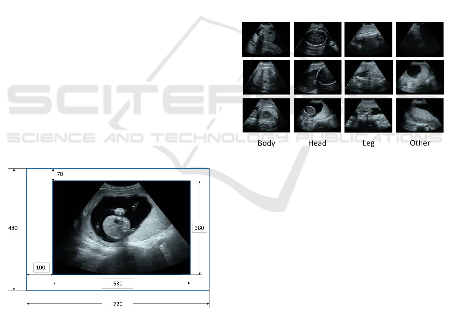
Approximately 20,000 frames are extracted from

each video. The size of the image (frame) is 720 * 480

(pixels). Note that in this research, in order to hide the

patients’ personal information and examination

information, as shown in Fig. 1, only the ultrasound

image part is extructed as ROI (region of interest) and

used for the experiments.

Figure 1: Original ultrasound image and ROI.

2.2 Image Labels

We assigned four classes (head, body, legs, and

others) for all the ultrasound images. Examples of the

four classes are shown in Fig. 2. For non-experts, the

three classes: head, body and leg are easy to identify

and locate; that’s why we assign the four classes (the

three classes + others). Though the class of each

image is assigned by non-experts, the guidance of the

doctors and related reference (Shinzi. T, 2014) helps us

make acceptable annotations.

󰈆 Head

The frame in which the skull is certainly visible as

well as its previous and next frames.

The head top is observed as a small circle.

󰈇 Body

The frame in which the gastrocytes are visible in

circles with almost uniform gray and the spine exists

as well as its previous and next frames.

󰈈 leg

There is a thick, straight white line. The pelvis and

two legs are visible.

󰈉 Other

Other cannot be classified by the above-mentioned

three classes.

Figure 2: Criteria for classification.

Also, images in which multiple objects appear are

eliminated from the training images.

Totally, 21,110 frames with the head label, 23,300

with the body label, and 14,887 with the leg label.

Based on these data, we used 10,000 frames for

training and others for testing. From the training

frames, 2,000 frames are used for validation.

2.3 Data Augmentation

We expand the number of frames using data

augmentation for the images labelled in Section 2.2.

Types of augmentation are: moving to the left / right

direction, enlarging / reducing (Oquab..M, 2014),

(Razavian. A, 2014). Rotation and color tone

correction etc. are not carried out. Horizontal

movement, enlargement / reduction are performed

randomly, so that the number of deta is increased

about five times as many as the original frame number.

ICPRAM 2019 - 8th International Conference on Pattern Recognition Applications and Methods

182

3 ALGORITHM

3.1 Overview

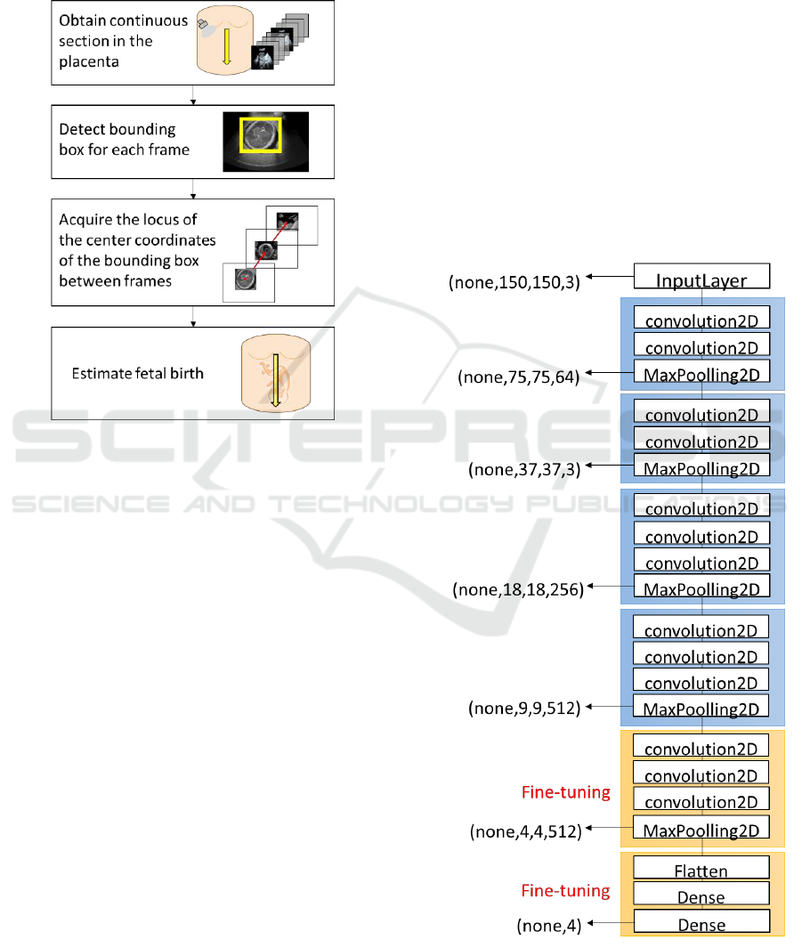
This section overviews the proposed method.

Figure 3: Overview of our proposed method.

Figure 3 shows an overview of the proposed method.

First, continuous cross sections are extracted from the

maternal body of a pregnant woman. Clustering is

performed in each frame, and Grad_CAM

(Ramprasaath. R., 2017) is applied to the clustering

results. The bounding box is generated at the image’s

part with large gradient. The centeral coordinates of

the detected bounding box are obtained with respect

to the continuous cross section. Noise reduction is

performed for the trajectory at that time, and the fetal

birth position in the Uteras is estimated.

3.2 Network

We aim to accurately classify each frame. We utilize

the basic feature extraction layer VGG_16 (Karen S,

2014). As shown in Fig. 4, in order to ensure the

convergence of learning, fine tuning using

ImageNet's weight is performed. We learn the

multilayer perceptron of the full coupling layers of

VGG 16 and its previous convolution layers.

VGG 16 is a convolutional New Jersey network

consisting of a total of 16 layers of 13 convolution

layers and 3 full layers proposed by ILSVRC

(ImageNet Large Scale Visual Recognition

Challenge) in 2014. It has a simple structure which is

not very different from a general convolution neural

net with only a large number of layers. As shown in

Fig. 4, fine tuning is performed from the 



layer to





layer of the convolution layers. In the

convolution neural network, shallow layers tend to

extract edges and blobs. On the other hand, deep

layers tend to extract features unique to specific

object that were learnt. In that case, the general-

purpose feature extractor of the shallow layer is fixed

as it is, and the current fetal ultrasound image of the

deep layer weight is relearned. For all binding layers,

four classes are output as "head", "stomach", "leg",

"other". SGD (Stochastic Gradient Descent) is used

for optimization in learning. In the descent method it

is impossible to escape from the problem of local

convergence. However, SGD tends to escape the local

convergence easily due to the influence of random

Figure 4: Model layer (VGG16).

Detecting a Fetus in Ultrasound Images using Grad CAM and Locating the Fetus in the Uterus

183

numbers and it is easy to globally converge (Leon. B,

1991).

Furthermore, our data set includes images of wide

ranges (including head edges and centers) of the head,

abdomen (body) and leg. We do not aim at extracting

some deterministic features, instead, extracting rough

features that likely describes each class.

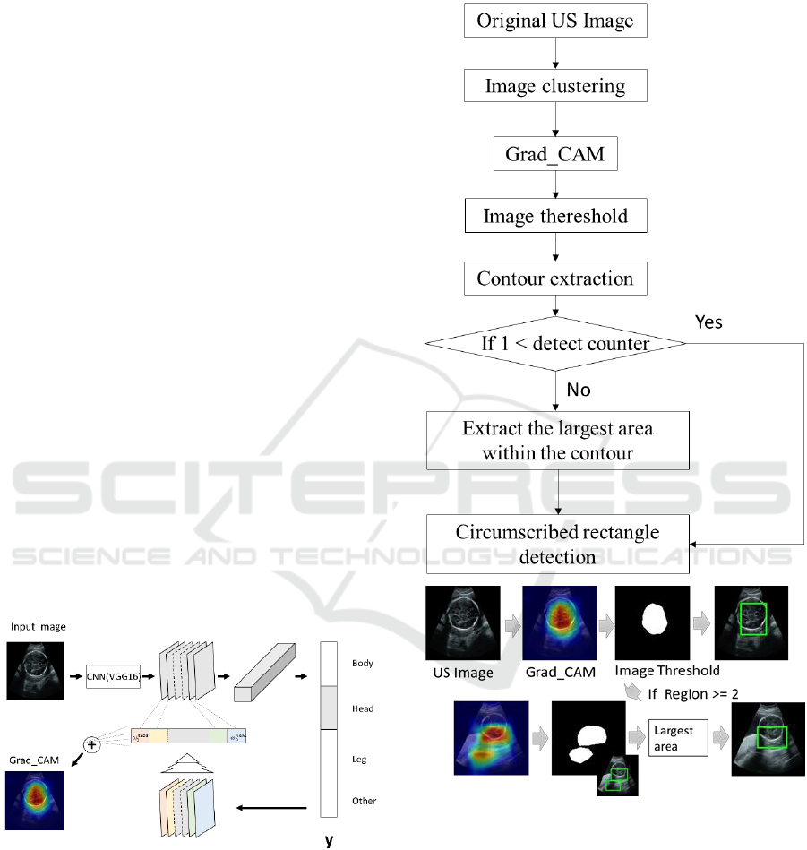
3.3 Grad_CAM

Grad-CAM uses the gradient information flowing

into the last convolutional layer of the CNN to let the

viewer understand the importance of each neuron for

a region of interest. An overview is shown in Fig. 5.

The convolution neural network is roughly divided

into two parts. The first one is a feature extracting part

where the convolution layer and the pooling layer are

stacked in layers, and the second part is an identifying

part which receives the feature output and performs

supervised learning by collating it with the class label.

The identification part usually consists of a multilayer

neural network of all connections, and the final layer

is a soft max layer that converts the feature quantity

to the probability score of each class. The image

points that have a large influence on the probability

score for each class are identified by gradient

averaging. Gradient is a coefficient that indicates the

magnitude of the change that occurs in the probability

score when a tiny change is added to a certain image

part in the feature amount map. The gradient of the

probability score is also large for the image part

where the influence on the class determination is

large.

Figure 5: Conceptual diagram of Grad_CAM.

3.4 Region Localization

By using Grad_CAM, it is possible to visualize which

features in the cross section contribute to judging the

class. Also, since our data set has a wide range in each

class, the visualized features indicate the "likeness"

obtained by the learned network. The area obtained

by this indicator is detected as a bounding box. The

detection of the bounding box is performed according

to Fig. 6.

Figure 6: Detecting bounding boxes.

First, the learned network created in Section 3.2 is

applied to the original ultrasound image. For each

image, a class label (head, body, legs, etc.) is assigned.

After that, the Grad_CAM corresponding to each

label is used. Images’ parts are identified based on

averaging the gradient and the largest probability

score. Meanwhile, gradient equal to or less than the

threshold is removed by Eq (1).

  

(1)

ICPRAM 2019 - 8th International Conference on Pattern Recognition Applications and Methods

184

where max indicates the maximum value of the

differential coefficient obtained by Grad_CAM for

each image. Note that in Eq. (1), half of the

differential value with respect to the maximum value

is set as the threshold (range). Binarization is

performed using this threshold. In the obtained binary

image, contours are extracted. After then, the

rectangle circumscribing the extracted contour is

obtainnd(Suzuki S, 1985). If the number of the

detected contours (detect counter in Fig. 6) is one, that

contour is detected. If , the

largest detected box is chosen as the final result.

3.5 Object Position Estimation in

Image

The position of the fetus in the image is estimated

using the bounding boxes of each image obtained in

Section 3.4. An example of the image acquisition is

shown in Fig. 7.

Figure 7: Examples of acquiring consecutive frames.

In each image, the bounding box for the detected

object and the central coordinates of the bounding

box are obtained. The central coordinates of the

bounding boxes are obtained for all the continuous

cross sections so that the trajectory of the central point

is obtained. Here, the bounding box is extracted only

when the class labels are head, body, or legs. In case

of “other” label, accurate features are not obtained in

the learning stage. Also, when locating the fetus, the

fetus does not appear in the cross section in many

cases. The bounding box of the "other" class works as

noisy information for locating the fetus; thereby, the

bounding box is not generated.

In addition, the trajectories of the centeral coordinates

of the bounding box detected only by the head, body,

and legs may contain noise due to erroneous detection.

To eliminate this false detection case, noise removed

is performed according to the following procedure.

①Calculate the mean



) of all the images

②Calculate standard deviation (



) of all the images













 











(2)

③Remove noise outside the range of Eq. (3)





 







 



(3)

where a in Eq. (2) and (3) indicate the centeral

coordinates (x, y), n indicates the total number of

frames. The centeral line obtained by this result can

be considerd as the area where the fetus exists.

4 EXPERIMENTS

In this chapter, we present experimental results. First,

the learning results of the network illustrated in

Section 3.2 are explained in Section 4.1. Evaluation

for Section 3.3 is performed in Section 4.2.

Evaluation for Section 3.4 is performed in Section 4.3.

4.1 Classification of Fetal Parts

VGG 16 was used for learning. Fine tuning was

carried out with the total binding layer and the

convolution layer. We prepared 8,000 frames for

training and 2,000 frames for validation. The left and

right movement and scaling were used for the data

augmentation. Batch size is set to 8, and epoch is 30.

The learning rate is set to 0.001. The transition of the

learning result is shown in Fig. 8. The horizontal axis

of Fig. 8 shows epoch. The left vertical axis shows

learning loss and the right vertical axis shows

accuracy

The recall ratio is shown in Table 1. The test data are

combined by 2000 frames (500 frames / class) which

are not used for training.

Figure 8: Relationship between loss and accuracy.

Detecting a Fetus in Ultrasound Images using Grad CAM and Locating the Fetus in the Uterus

185

Table 1: Recall of each part.

Class

Recall

Body

94.0

Head

99.6

Leg

99.8

Other

72.6

High recall ratios were obtained for the head, body

and leg except for “other”. We believe that the other

recall rates are low due to the diversity of the features.

In this study, we estimate the fetal position in the

image,; thereby, we believe that the low recall rate of

the “other” class does not significantly affect the

estimation of feal position.

The confusion matrix of each class is shown in Table

Table 2: Confusion matrix.

body

head

leg

other

body

470

head

498

leg

499

other

363

From Table 2, the “other” class is likely to be

confused with the other classes. It indicates the

uncertainty of the “Other” class. The images of the

“Other” class are easily misclassified by body, head

and leg, which results in a low recall rate.

4.2 Result of Region Localization

An example of the heat map generated by Grad_CAM

is shown in Fig. 9.

The three classes except the “other” class accurately

indicate the part of the fetus. Even from the

classification of the non-experts who are not familiar

with ultrasound images, we could extract the features

of the target part and show them in the form of a heat

map. However, due to the diversity of the “other”

class, the heat map of the “other” class cannot be

easily distinguished. Thus, the VGG-16 network

cannot learn the feature of the “other” class very well.

4.3 Result of Fetal Parts’ Position

Estimation in Images

In this section, we describe the results of applying the

algorithm in Section 3.4. In the experiment, a

phantom (41905-000 US-7 fetal ultrasound

diagnostic phantom "SPACEFAN-ST") of a fetal

Figure 9: Feature extraction using Grad_CAM.

pregnancy medical exercise practice model was used

to fix the condition. In Section 4.3.1, experiments

were conducted on the data acquired as shown in Fig.

7 with the fetal fixed in the center of the image. In

Section 4.3.2, in addition to the image acquired in

4.3.1, the case where the fetal is shifted to the right in

the image and the case where it is shifted to the left in

the image are compared.

4.3.1 A Case in Which the Fetus is Placed in

the Center

In this section, we present the results when we

continuously acquire images from the maternal one

end to the other end while the fetus is at the middle of

the image. Feature extraction of each frame was

performed, and the trajectory of the centeral

coordinates of the generated bounding boxes was

acquired.

Figure 10 shows the results where the horizontal axis

indicates the number of frames, and the vertical axis

indicates the depth for the row direction of the

bounding box. In addition, since the input image to be

learnt is resized to (150, 150), the input image for fetal

part detection is also resized to (150, 150). That is, the

vertical axis of Fig. 9 corresponds to the row of the

image. The number of frames of the continuous cross

section is 761.

ICPRAM 2019 - 8th International Conference on Pattern Recognition Applications and Methods

186

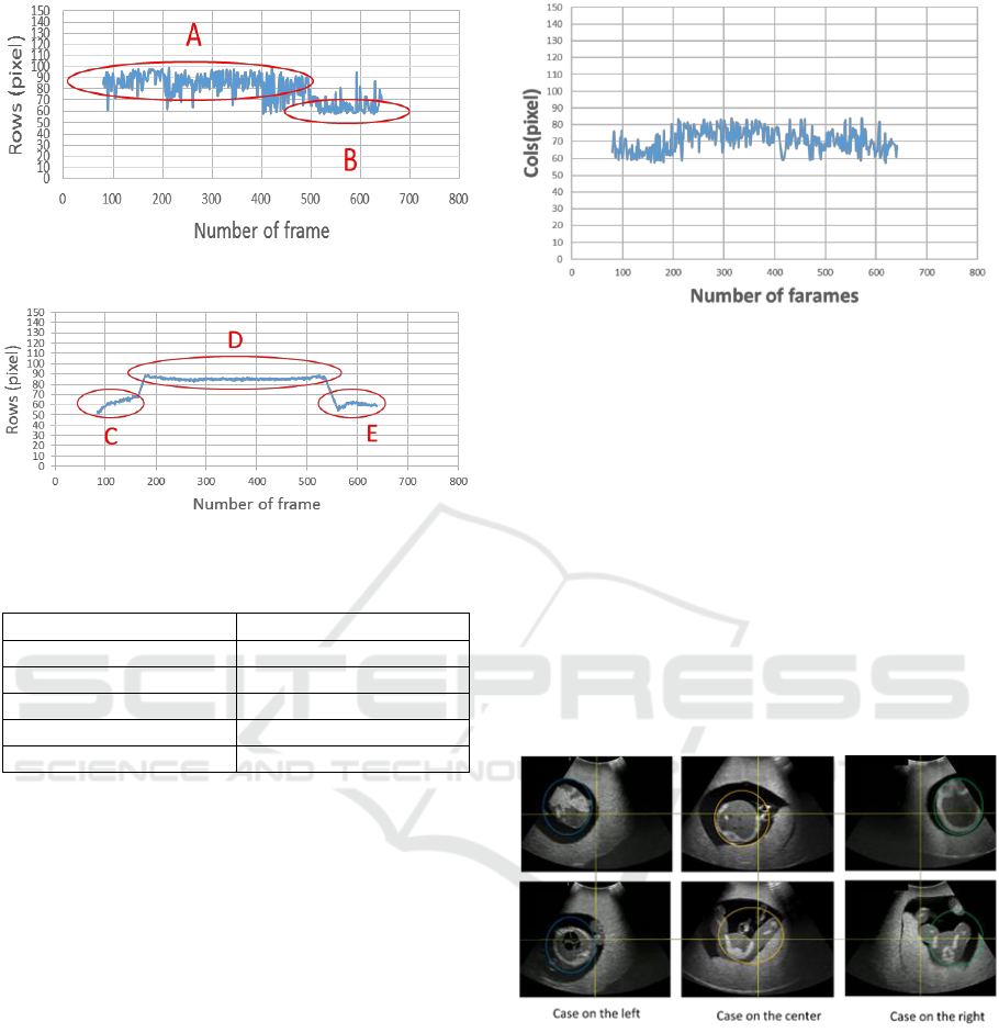
Figure 10: Trajectory of the fetal area(Row).

Figure 11: Shows the Ground truth of Fig. 10.

Table 3: Average of A to E regions in Fig. 10 and 11.

Area

Average depth

84.9

66.2

62.4

85.3

62.4

Figure 11 shows the ground truth of Fig. 10. The

ground truth is created by the bounding box manually

extracted from the data used in Fig. 10.

Furthermore, Fig. 10 is divided into A and B having

different depths. Figure 11 is similarly divided into C

to E having different depths. The average depths of A

to E are shown in the Table 3. In Fig. 11, C,D and E

correspoud to leg, body, and head, respectivery. In

Fig. 10, the depth of the head region is lost. However,

when comparing A and D, B and E, the errors

between the corresponding areas are very small. On

the other hand, the reason why the head cannot be

detected accurately is that the fetal model "phantom"

has little difference between the head and body, while

the head and body of the real fetus is different.

Next, the result in the left-right direction (cols

direction) is shown in Figure 12.

Figure 12: Trajectory of the fetal area (cols).

As in Fig. 9, the result of Fig. 12 can also show the

center of the bounding box in the images as a

trajectory. From these results, it can be said that it is

possible to estimate how the fetal central axis (fetal

position) is located inside the mother's body.

4.3.2 The Case Where the Fetus is Shifted to

the Left and Right

In this section, when the fetus is shifted to the left and

right of the image in each frame, the trajectory of the

fetal is acquired. The obtained results are compared

with the results shown in Sec. 4.3.1, in which the fetus

is at the “center”. The three kinds of images to be

used are shown in Fig. 13.

Figure 13: Image examples: right, center, left.

As shown in Fig. 13, the images are acquired

continuously. The left column contains 769 frames,

the central column contains 761 frames, and the right

column contains 528 frames. As in Section 4.3.1, the

trajectories of all the three patterns in Fig. 13 are

visualized in Fig. 14.

Detecting a Fetus in Ultrasound Images using Grad CAM and Locating the Fetus in the Uterus

187

Figure 14: Trajectory of fetal areas (comparison of right,

left, center).

If three approximate curves are obtained, it is possible

to visualize the respective positional relationships.

The approximate curve obtained by using the least

squares method for each line is shown in Table 3. The

averages (



) and standard deviations (



) of each

trajectory are also listed in Table 4.

Table 4: Approximate curve parameters.











Right

0.0134

90.129

94.362

9.020

Center

0.0042

69.064

70.570

6.524

Left

-0.0011

56.698

56.377

4.145

In Table 4, a is the slope and b is the intercept. At this

time, since the inclination is a small value, it is not

taken into consideration. It can be seen that the

difference between the central trajectory and the

intersection of the left trajectory is narrower than the

difference between the central and the right intercept.

The reason on why the orange and blue lines are close

to each other is due to the fact that the continuous

image acquired so as to pass through the center is

slightly leftward as shown in Fig. 12.

The standard deviation values obtained from the

approximate curves of the loci of "center", "left", and

"right" were 70.57 ± 6.52, 56.38 ± 4.15, 94.36 ± 9.02

respectively. The average indicates the distance

between the fetuses, and the standard deviation

indicates the blur of the central axis of the fetus. The

difference in position appeared in all that, but the

central axis was blurred on the right.

In the future it will be necessary to increase the range

of image augmentation in the left and right direction

and to reduce blurring of the fetal posture. In addition,

it is necessary to improve accuracy by using previous

and next frames.

Let us consider the right case (green), from the results

of the Table 3, the value of σ_a is much larger than

center and left cases, mainly because it is often mis-

classified as “Other” class. 398 frames of all 528

frames are judged as "Other". It is caused by the fact

that many images were missing more than half when

acquiring a continuous cross section. In order to

classify accurately even when it is missing, it is

necessary to increase the amount of movement left

and right during augmentation, and to increase the

number of defect images in a pseudo manner.

However, from the results of Fig. 13 it was suggested

that the trajectory of the fetus could be supplemented

to some extent at present.

4.4 Future Work

The proposed method detects, a fetal region from the

result of Grad_CAM, and a bounding box is

generated, but there is no result that proves it is a

correct answer. It is necessary to show the validity of

the proposed method more quantitatively by having

partnership with a doctor and evaluating accurate

detection by the procedure.

Also, it is necessary to perform comparative

verification of other deep learning frameworks such

as Alex_Net and Res_Net.

In addition, when multiple fetal regions are detected,

the region with the maximal area is outputted. Based

on the results of a few previous frames, the accuracy

of outputting the region could get higher.

We could estimate the position of the fetus in the

image by the proposed method and the fetal position

obtained from the continuous images. Based on these

results, it was difficult to fully determine the standard

cross section for estimating the weight of the fetal in

the past, but it is thought that measurement becomes

easy by detecting the center of the fetal. In addition,

3D ultrasonic machines are also being used more

frequently in recent years.

As a related study, research using 3D data such as

Nambure A. et al.’s research (Nambure A, 2018) on

3D fetal brain’s important feature extraction is

increasing. Furthermore, 3D fetal examination relies

on medical doctors’ experiences more than 2D

examination. The proposed method can obtain the

fetal depth in images; therefore, the estimated results

of the proposed method can be applied to automatic

measure using 3D US machine in the near future.

5 CONCLUSIONS

This paper has proposed an automatic method for

estimating fetal position from ultrasound images

based on classification and detection of different fetal

parts in ultrasound images. Fine tuning is performed

in the ultrasound images to be used for fetal

ICPRAM 2019 - 8th International Conference on Pattern Recognition Applications and Methods

188

examination using CNN, and classification of four

classes is realized. Based on the obtained learning

result and the gradient of the feature obtained by Grad

Cam, a bounding box is generated at the image’s part

with the largest gradient. The trajectory of the center

of the bounding box in each image is obtained as the

position of the fetus. Experimental results are as

follows.

The fetal four class recall ratios were 99.6% for

head, 99.4% for body, 99.8% for legs, 72.6% for legs.

The trajectories obtained from the fetus present in

“left”, “center”, “right” in the images show the above-

mentioned geometrical relationship.

In the estimation of the depth of the fetus,

although the problem remains in estimating the depth

of the head part, the accuracy of estimating the depth

of the fetal body and the leg part is high. In the future,

it is necessary to improve accuracy by using other

deep learning networks and previous and latter

relative frames.

These results indicate that the estimated fetal

position coincides with the actual position very well,

which can be used as the first step for automatic fetal

examination by robotic systems.

ACKNOWLEDGEMENTS

This research is a collaborative study with Ikeda and

Rattan in Iwata laboratory at Waseda University.

Iwata and colleagues are developing TENANG robot

for pregnant women's ultrasound examination.

REFERENCES

Christian F, Konstantinos K, Jacqueline M, Tara P, et. al.

2017, Sononet: real-time detection and localisation of

fetal standard scan planes in freehand ultrasound. IEEE

Transactions on Medical Imaging, 36(11):2204{2215.

Gull I, Fait G, Har-Toov J, et al. 2002, Prediction of Fetal

Weight by Ultrasound: the Contribution of Additional

Examiners. Ultrasound in Obstetrics and Gynecology,

vol. 20, no. 1, pp. 57-60.

Hadlock F. P, Deter R.L, Harrist R.B, Park S.K. 1983,

Computer Assisted Analysis of Fetal Age in the Third

Trimester Using Multiple Fetal Growth Parameters. J

Clin Ultrasound, vol. 11, pp. 313-316.

Hadlock F. P, Deter R., Carpenter R, et.al. 1981, Estimating

Fetal Age: Effect of Head Shape on BPD, American

Journal of Roentgenology. vol. 137, no. 1, pp. 83-85.

Karen S and Andrew Z. 2014, Very deep convolutional

networks for large-scale image recognition. In ICLR,

International Conference on Learning Representations

2015.

Leon. B.199, Stochastic gradient learning in neural

networks. In Proceedings of Neuro-Nˆımes. EC2.

Namburete A, Xie W, Yaqub M, Zisserman A. 2018, Fully-

automated alignment of 3D fetal brain ultrasound to a

canonical reference space using multi-task learning.

Med Image Analysis, vol46, pp.1-14.

Nicolas T, Bishesh K. et al, 2018, Weakly Supervised

Localisation for Fetal Ultrasound Images, 4th

International Workshop, DLMIA 2018, and 8th

International Workshop, ML-CDS 2018, pp.192-200.

Oquab, M., Bottou L, Laptev, I,(2014) Learning and

transferring mid-level image representations using

convolutional neural networks, Proc. CVPR, pp. 1717-

1724.

Razavian, A., Azizpour, H. and Sullivan, 2014, J.: CNN

features off-the-shelf: An astounding baseline for

recognition, Proc. CVPR, pp. 512-519.

Shinzi. T. 2014, Sanka Chouonpa Kensa (Obstetric

ultrasound examination). Japan: Igaku shyoin, p.58.

Suzuki, S, Abe, K., 1985. Topological Structural Analysis

of Digitized Binary Images by Border Following.

CVGIP 30 1, pp 32-46.

Ramprasaath R. Selvaraju, Michael C, et al. 2017, Grad-

CAM: Visual Explanations from Deep Networks via

Gradient-based Localization. IEEE International

Conference on Computer Vision (ICCV), pp. 618-626.

Yuanwei Li, Bishesh K, Benjamin H, 2018, Standard Plane

Detection in 3D Fetal Ultrasound Using an Iterative

Transformation Network. MICCAI 2018: Medical

Image Computing and Computer Assisted Intervention

– MICCAI, vol11070, pp 392-400.

Detecting a Fetus in Ultrasound Images using Grad CAM and Locating the Fetus in the Uterus

189