Design Guidelines for Feature Model Construction:
Exploring the Relationship between Feature Model Structure
and Structural Complexity
Xin Zhao and Jeff Gray
Department of Computer Science, University of Alabama, Tuscaloosa, AL, U.S.A.
Keywords: Model-driven Engineering, Feature Modeling, Model Complexity, Data Mining.
Abstract: Software Product Lines (SPLs) play an important role in the context of large-scale production of software
families. Feature models (FMs) are essential in SPLs by representing all the commonalities and variabilities
in a product line. Currently, several tools support automated analysis of FMs, such as checking the consistency
of FMs and counting the valid configurations of a product line. Although these tools greatly reduce the
complexity of FM analysis, FM design is often performed manually, thus being prone to bad design choices
in the domain analysis phase. This paper reports on our work to improve FM qualities from the exploration
of the relationship between FM structure and structural complexity. By performing two common operations
(i.e., consistency checking and counting valid configurations on FMs with different sizes and structures), we
collected the time that an automated tool needs to finish these operations. Then, we applied data mining
approaches to explore the relationship between FM structure and structural complexity. In addition, we
provide guidelines for designing FMs based on our observations.
1 INTRODUCTION
Off-the-shelf software is often complex, hard to
debug and burdensome to maintain because it tries to
provide a one-size-fits-all solution. In order to deal
with software generalization, Software Product Lines
(SPLs) (Clements and Northrop, 2002) emerged in
the late 1960s. SPLs focus software development on
reusable parts to provide flexible product
configurations based on individual needs. Instead of
software development as a whole system from
requirements analyses to testing, SPL divides
software into several standardized parts that are easier
to check and test compared with integrated systems.
SPLs reduce development cost and time before they
are released to the market because developers do not
need to design and develop each product from scratch
(Apel et al., 2016). Creating different products for
different needs is simplified to the selection of
options from common functional assets.
A feature model (FM) is a compact representation
of all the software products in terms of features in an
SPL. In this paper, we provide design guidelines for
FM construction from the exploration of the
relationship between FM structure and complexity.
FM structure refers to the structure of a feature
diagram - a graphical representation of a FM. FM
structural complexity is the complexity of a FM
representation across several operations. We use the
execution time for FM analysis operations to measure
the structural complexity of a model. By examining
the relationship between a FM’s structure and its
structural complexity, we explore the internal
association among these two factors, thus providing
guidelines for FM construction to domain analysts.
The core contributions of this paper include the
following:
 Application of data mining approaches to explore
the relationship between a FM’s structure and
structural complexity;
 A set of design guidelines for FM construction to
domain analysts.
This paper is organized as follows. In Section 2, we
introduce background information about FMs and the
evaluation of FM structural complexity. Section 3
presents a running example to explain the purpose of
our work. In Section 4, we give an introduction to our
experimental setup and in Section 5, we summarize
and analyze the results of our experiment, and provide
our guideliens for FM construction. Section 6
Zhao, X. and Gray, J.
Design Guidelines for Feature Model Construction: Exploring the Relationship between Feature Model Structure and Structural Complexity.
DOI: 10.5220/0007388703230331
In Proceedings of the 7th International Conference on Model-Driven Engineering and Software Development (MODELSWARD 2019), pages 323-331
ISBN: 978-989-758-358-2
Copyright
c
 2019 by SCITEPRESS – Science and Technology Publications, Lda. All rights reserved
323

discusses the threats to validity in our work. In
Section 7, we identify related work in the literature.
We conclude this paper and propose future work in
Section 8.
2 BACKGROUND
In this section, we introduce concepts about feature
model, one approach used to evaluate the feature
model structural complexity and two data mining
approaches applied in this paper.
2.1 Feature Model
In a feature model, features have different
characteristics. If a feature is expected to appear in
every product in a product line, this feature is
mandatory. Otherwise is optional. If a feature acts as
an interface, it is an abstract feature. Otherwise, it is
a concrete feature. Figure 1 shows a feature model for
a simple cellphone SPL.
Figure 1: A feature model for a cellphone SPL.
A feature model is usually organized as a tree
structure. Similar to other tree structures, a feature
diagram incorporates the concepts of parent and child
nodes. If a feature is the child of another feature, the
child feature can only be selected when its parent
feature is chosen. When several children are selected
from a single parent node at the same time, we define
this relationship as OR. When only one child node is
allowed to be selected among several children, we
define this relationship as XOR (eXclusive OR). In
Figure 1, feature Screen and feature
White/Black, Color and Resolution consist
of an XOR group. Features Media, Music and
Photo form an OR group.
2.2 Complexity Evaluation
Štuikys and Damasevicius (2009) proposed
Compound Complexity (CC) to assess the structural
complexity of a feature model, shown as follows:
CC = NF + 1/9 * NM
2
+ 2/9 * NO
2
+
1/3 * XOR
2
+ 1/3 * OR
2
+ 1/3 * N
C
2
(1)
In the formula above, NF is the number of features;
NM is the number of mandatory features; NO is the
number of optional features; XOR is the number of
exclusive OR groups; OR is the number of OR
groups, and NC is the number of constraints. The
calculation formula and the constants in Equation (1)
are based on criticism of Metcalfe’s law (Briscoe et
al., 2006). Metcalfe’s law (Shapiro et al., 1998) is a
statement showing that the value of network
communications is proportional to the square of the
number of connected users in the system. However,
whether the weight assigned to each metric is
accurate needs further validation both from a
theoretical and empirical perspective.
2.3 Data Mining
2.3.1 Linear Regression
Regression is a data mining technique for predicting
continuous values. It estimates the conditional
expectation of a dependent variable given the
independent variables. There are several types of
regression, such as linear regression, logistic
regression and non-linear regression. Multiple linear
regression takes the form:
 = β
1
* 
1
+ β
2
* 
2
+ β
3
* 
3

…
+ β
n
* 
n
+ 
(2)
Multiple linear regression tries to model the
relationship between one dependent variable and two
or more independent variables by making them fit
into a linear equation to observe the pattern. For
example, if we want to observe whether individual
income has a relationship between one’s education
background, living place and working experience, we
can apply multiple linear regression to the model,
setting individual income as the dependent variable
and other factors as independent variables. In this
paper, we first apply multiple linear regression to
explore the relationship between feature model
structure and its structural complexity.
2.3.2 Support Vector Machine
A Support Vector Machine (SVM) is a supervised
learning model in machine learning and data mining
MODELSWARD 2019 - 7th International Conference on Model-Driven Engineering and Software Development
324

for data classification and regression analyses,
proposed by Vladimir Vapnik and his colleagues in
1992 (Boser et al., 1992). SVM is widely used in data
classification and data regression. In this paper, we
use SVM in regression analysis through Support
Vector Regression (SVR).
Given a data set, SVR maps input examples into a
high dimensional feature space and performs
regression in that space. SVM regression performs
linear regression proposed by Vapnik. By calculating
the empirical risks of the loss function, the original
problem could be solved through an optimization
problem (Boser et al., 1992).
When we apply SVM for different regression
problems, we need different kernel functions. The
selection of a kernel function plays an important role
in the accuracy of the results. However, constructing
a kernel function for a specific problem is still a
challenge (Su and Ding, 2006). The most frequently
used kernel functions are polynomial kernel function,
radial basis function kernel (RBF kernel function) and
Sigmoid kernel function. In this paper, we apply a
polynomial kernel function in our experiment.
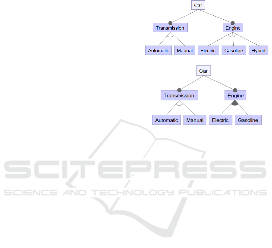
3 MOTIVATING EXAMPLE
Consider an automotive product line with two basic
necessary functions – Transmission (either
Automatic or Manual) and Engine (either Electric,
Gasoline, or both). From Figure 2, we see that the
solutions are different. Feature model 2.b applies
feature group notation – OR, whereas feature model
2.a simply lists all the sub-features according to the
requirements (Hybrid means the car could use both
electric power and gasoline).
Among feature model 2.a and 2.b, which one is
preferred? The answer to this simple question is not
as easy as it seems, especially when the number of
features in a feature model is large. There are many
metrics proposed by researchers to evaluate a feature
model. In Bezerra’s work (Bezerra et al., 2015),
although the authors summarized more than 40
metrics to evaluate a feature model in different
characteristics, choosing the best metric is still
challenging for developers. For these metrics, most
are statistical descriptions of feature models, such as
the number of features, and the number of constraints.
However, there is not a clear understanding on how
to analyze a combination of these metrics. Although
Stuikys et al. (Štuikys and Damaševičius, 2009) try to
solve this problem by providing three types of
complexities (i.e., structural complexity, compound
complexity and cognitive complexity), they did not
consider whether different metrics have different
weights when calculating feature model complexity.
Figure 2.a
Figure 2.b
Figure 2: Two different feature model designs for the same
problem description.
4 EXPERIMENTAL SETUP
In this section, we discuss our experimental setup. We
start with defining our research questions, then we
summarize the methodologies we used to answer the
research questions. We also introduce the execution
environment and tools used in this work. The results
of our experimental data are available at the following
URL: http://bit.ly/feature-data.
4.1 Research Questions
Motivated by the example introduced in Section 3, we
define our research questions as follows:
 Research Question 1 (RQ1): What is the
relationship between feature model structure and
structural complexity?
 Research Question 2 (RQ2): What guidelines
can be recommended for feature model
construction based on observations from RQ1?
4.2 Experiment Design
Given a feature model, assuming that the model
satisfies all the requirements, we are interested in
whether the structure of the feature model affects its
structural complexity. For example, the feature
Design Guidelines for Feature Model Construction: Exploring the Relationship between Feature Model Structure and Structural Complexity
325

models shown in Figures 2.a and 2.b both represent
the same software product line. Feature model 2.b
uses fewer features, but adopts an OR group instead
of a XOR group. What is the consequence of this
modification? Will the increase of OR groups in a
feature model also increase the structural complexity,
even if the total number of features decrease?
In this paper, we chose seven independent
variables:
 
1
: The number of total features (TF);
 
2
: The number of mandatory features (MF);
 
3
: The number of optional features (OF);
 
4
: The number of OR groups (OR);
 
5
: The number of XOR groups (XOR);
 
6
: The number of total features that are in either
OR group or XOR group (NG) ;
 
7
: The number of constraints (NC).
There are two reasons why we selected these seven
metrics. First, as integer values, these metrics are the
most basic structural measuring metrics; second, the
calculation of these metrics are provided by an
automated tool we used in our experiment (please see
Section 4.4 for details). For a feature model, the value
of 
1
to 
7
is easy to obtain by analyzing the FMs.
In order to obtain the value of y corresponding to
each set of 
i
, we adopted the approach proposed by
Pohl et al., (2013). In their approach, they applied
width measures from graph theory to identify the
structural complexity of feature models. By setting a
feature model to automated analysis, they collected
the time consumed by their analysis tool to finish the
operations. They used the time spent as an indicator
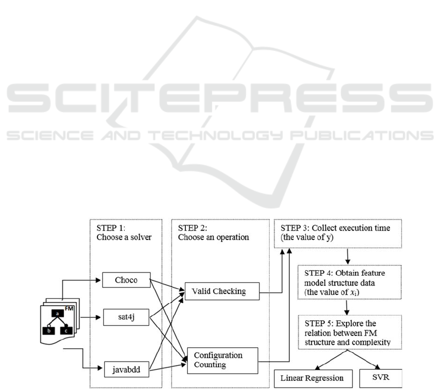
for structural complexity of a feature model. In our
approach, we chose three solvers to perform two
operations. The three solvers are Choco (Jussien et
al., 2008), sat4j (Le Berre and Parrain, 2010) and
Javabdd (Whaley, 2007). The two operations check
whether a feature model is valid and count the number
of valid configurations.
After the collection of 
i
and its corresponding
feature model structural complexity , we need to
find the relationship (i.e., the value of coefficients for
each 
i
) between feature model structure and its
structural complexity. We apply two approaches:
multiple linear regression and SVM. The process of
our experiment is shown in Figure 3.
4.3 Experiment Execution
Our experiment is executed on a desktop with an Intel
Core i7 – 4790 CPU at 3.60 GHz and 8 GB RAM.
The operating system is Windows 7 64-bit. Each
operation on each task had a timeout of 3600s.
4.4 Tool and Feature Model Repository
In order to obtain the FM structural complexity, we
adopted the automated tool from Pohl’s work. The
automated tool provides automated analysis of FMs,
such as valid checking, valid configuration counting,
and listing all the valid configurations. The tool is
available at (CoFFeMAP, 2018). In order to obtain
the feature structure information, we applied SPLOT
(Software Product Line Online Tool), which is an
online system for SPL editing and analysis
(Mendonca et al., 2009). We applied multiple linear
regression to explore the relationship between FM
structure and structural complexity. We used IBM
SPSS Statistics (SPSS, 2018), a widely used program
for statistical analysis in many areas. To apply SVM
for regression, we adopted a data mining tool called
Figure 3: Overview of experimental process.
MODELSWARD 2019 - 7th International Conference on Model-Driven Engineering and Software Development
326

Weka (Weka, 2018), which contains several machine
learning algorithms for data mining tasks. Both of
these two tools provide a graphical user interface.
5 RESULTS AND GUIDELINES
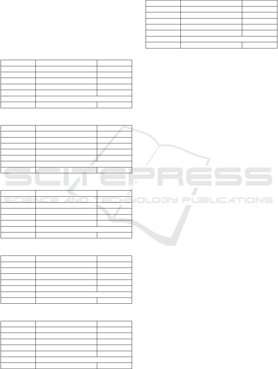
5.1 Experimental Results and Analyses
Table 1: LR for Choco performing valid checking.
Model Standardized Coefficients Sig.
TF 0.540 0.000
MF 0.062 0.304
OF -0.130 0.054
OR -0.025 0.628
XOR -0.017 0.747
NG Excluded Variable
NC 0.322 0.000
Table 2: LR for Choco performing configuration counting.
Model Standardized Coefficients Sig.
TF 0.219 0.130
MF -0.103 0.267
OF 0.141 0.054
OR 0.123 0.092
XOR -0.119 0.166
NG Excluded Variable
NC -0.037 0.581
Table 3: LR for sat4j performing valid checking.
Model Standardized Coefficients Sig.
TF 1.751 0.000
MF -0.424 0.000
OF -0.431 0.000
OR -0.200 0.000
XOR -0.418 0.000
NG Excluded Variable
NC 0.034 0.410
Table 4: LR for sat4j performing configuration counting.
Model Standardized Coefficients Sig.
TF 1.268 0.000
MF -0.799 0.000
OF -0.246 0.056
OR -0.125 0.254
XOR -0.589 0.009
NG Excluded Variable
NC -0.202 0.006
Table 5: LR for Javabdd performing valid checking.
Model Standardized Coefficients Sig.
TF 0.159 0.523
MF -0.097 0.479
OF 0.006 0.956
OR 0.065 0.440
XOR -0.192 0.708
NG Excluded Variable
NC 0.027 0.739
Table 6: LR for Javabdd performing configuration
counting.
Model Standardized Coefficients Sig.
TF 0.351 0.070
MF -0.113 0.279
OF -0.122 0.171
OR 0.535 0.000
XOR -0.023 0.806
NG Excluded Variable
NC -0.096 0.118
Tables 1 through 8 show our results for regression
analyses of all the FMs in our experiment (timeout
results are excluded). Tables 1 to 6 are the results
from multiple linear regressions executed in IBM
SPSS. Table 7 show the results from SVR performed
in Weka (kernel function is polynomial kernel and the
exponent is set to 1). Table 8 shows the results with
the same experimental setting as Table 7. However,
in Table 8, all FMs have only 10 features.
5.1.1 Multiple Linear Regression
From Tables 1 to 6, we can see that most of the results
we obtained from multiple linear regression have a
significant value larger than 0.05. Therefore, most of
the values are not statistically significant. One
explanation for this may be for a given FM, its
structure and structural complexity is not a linear
relationship. The number of FM features and FM
constraints always have a positive correlation with its
structural complexity. Thus, the more features and the
more constraints in an FM, the higher its structural
complexity.
The more mandatory features in an FM, the less
structural complexity it demonstrates, which seems
intuitive. Suppose in a FM, if all the features are
mandatory, then there will be only one possible valid
configuration – a configuration simply adds up all the
features without any variabilities. On the other hand,
if a FM has many variations, it will increase its
structural complexity.
From Tables 1 to 6, we can also observe that given
the same data, different solvers produce different
analysis results (compare with Table 1, Table 3 and
Table 5; Table 2, Table 4 and Table 6). It also
indicates that the structural complexity also relates to
the solver used. Our experimental data shows that
when performing the same tasks, Javabdd and sat4j
run faster than Choco. This finding is not related to
our analysis in this paper, but it may provide
developers with insights into tool selection with
regard to FM automated analysis.
Design Guidelines for Feature Model Construction: Exploring the Relationship between Feature Model Structure and Structural Complexity
327

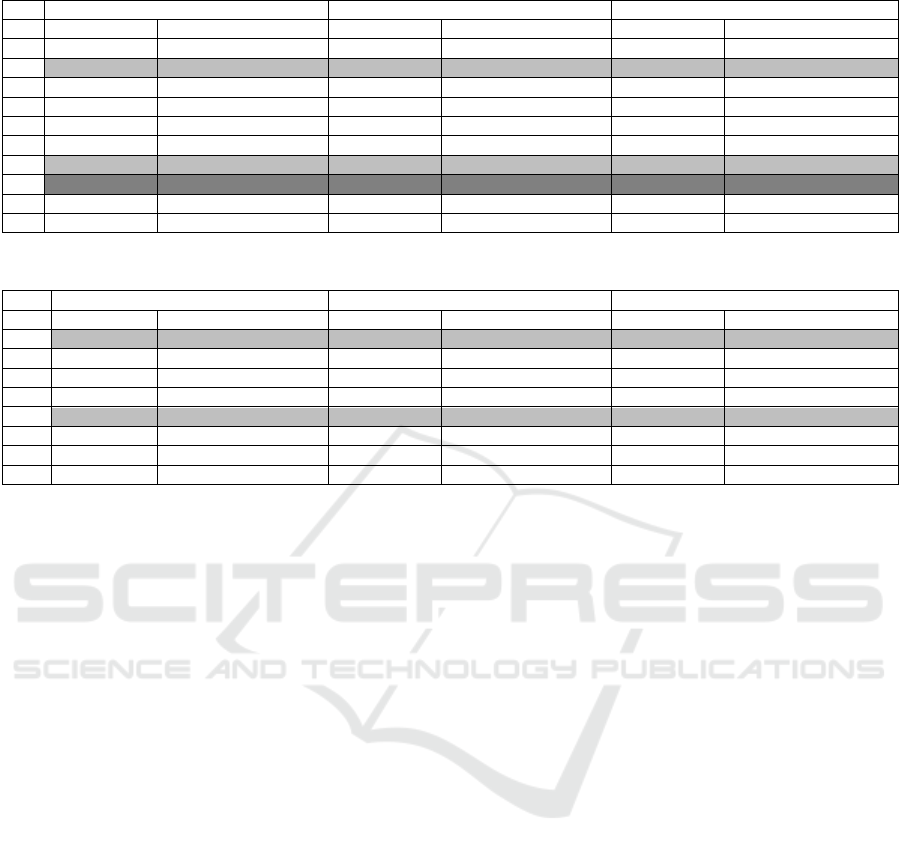
Table 7: Regression results based on SVR (MAE: Mean Absolute Error; MSE: Mean Squared Error).
Choco Sat4j Javabd
d
Valid Checking Configuration Counting Valid Checking Configuration Counting Valid Checking Configuration Counting
TF 0.327 0.0067 0.2522 0.0044 0.0308 0.0577
MF 0.1224 -0.0026 -0.0371 -0.0022 -0.0142 0.0039
OF 0.0582 0.006 -0.0807 0.0041 -0.0071 -0.0091
OR -0.1333 0.003 -0.0834 -0.0004 0.0096 0.046
XOR 0.0213 -0.0061 -0.0357 -0.0039 -0.0111 0.0485
NG 0.3597 0.0066 0.3786 0.0062 0.0607 0.0538
NC 0.268 -0.0063 0.0077 -0.0052 0.0016 -0.0007
MAE 0.0013 1.6306 0.0004 31.7262 0.0036 0
MSE 0.0021 12.402 0.0016 191.6283 0.0198 0.0001
Table 8: Regression results based on SVR given feature models with 10 features.
Choco Sat4j Javabd
d
Valid Checking Configuration Counting Valid Checking Configuration Counting Valid Checking Configuration Counting
MF -0.0437 -0.1927 -0.012 -0.0489 -0.1114 -0.0039
OF -0.0192 -0.1118 -0.2652 0.0178 -0.0765 0.0369
OR -0.0629 -0.0868 -0.3307 -0.0405 0.0216 0.1715
XOR -0.0973 -0.3744 -0.0364 -0.0246 -0.0569 -0.0485
NG 0.0628 0.3476 0.3119 0.035 0.2104 0.0833
NC -0.0141 0.0148 0.0695 -0.0195 0.0486 0.0104
MAE 0.0019 0.0025 0.0004 0.0069 0 0.0003
MSE 0.0027 0.0032 0.0005 0.0279 0 0.0005
5.1.2 SVR
From the results of Tables 1 to 6, we can see that the
relationship between a FM structure and structure
complexity is more complex than a pure linear
relationship. Based on this, we applied SVR for
regression and chose a non-linear kernel function for
regression. The results are shown in Table 7.
From Table 7, we can see that similar to the results
shown in Tables 1 to 6, the number of total features
and the number of grouped features (features either in
OR group or XOR group) have a positive correlation
with its structural complexity. Thus, the more
features/grouped features, the higher its structural
complexity. Although
Mean Absolute Error (MAE) and
Mean Squared Error (MSE) differs in each experiment,
this positive correlation does not change.
Another interesting observation from Table 7 is
that for the number of constraints in a FM, when the
FM executes a valid checking operation, the number
of constraints has a positive relationship with its
structural complexity. When the FM executes the task
of counting valid configurations, the number of
constraints has a negative relationship with its
structural complexity. One possible explanation for
this is during the execution of counting valid
configurations, the more constraints in an FM, the
fewer valid configurations available in a SPL, thus
making calculation time shorter than validation
checking.
Table 8 shows our experimental results when
executing all the tasks with different solvers on FMs
with 10 features. The purpose of this experiment is to
explore the relationship between FM structure and its
structural complexity when fixing the FM size. There
are two reasons why we chose models with 10
features:
 In the FM repository provided by SPLOT, there
are 83 FMs that have 10 features in the model. We
randomly chose 31 samples among these 83 FMs.
 Compared with FMs in other sizes, the experiment
results with 10 features are the most complete.
From Table 8, we can see that the number of
mandatory features has a negative correlation with the
structural complexity of a FM and the number of
grouped features has a positive correlation with the
structural complexity of a FM.
Compared with features in an OR group and in an
XOR group, we can see that features in an OR group
increase the structural complexity compared with
features in a XOR group. Another interesting finding
is that in different operations using different solvers,
the number of constraints plays different roles related
to the change of a FM’s structural complexity.
5.2 Guidelines for FM Construction
Based on the experimental results and analyses of the
previous section, we suggest the following guidelines
for FM construction:
MODELSWARD 2019 - 7th International Conference on Model-Driven Engineering and Software Development
328

 Use fewer features when possible. Both linear
regression and SVR support the conclusion that
the number of features in a FM always increases
the structural complexity when performing
automated analysis.
 Place fewer features in group notations when
possible. We also observe that when grouping
features in a FM, structural complexity is always
relatively higher.
 Choose an XOR group over an OR group when
both are options. An XOR group is better than an
OR group with regards to decreasing structural
complexity of a FM.
Although the guidelines seem intuitive, we validated
these guidelines from theoretical aspects. To our best
knowledge, this is the first study to confirm these
intuitive guidelines through experimentation.
6 THREATS TO VALIDITY
There exist several threats to validity in our study. In
this section, we discuss these threats from two
aspects: internal threats and external threats.
6.1 Internal Threats to Validity
Threats to internal validity compromise our
confidence in saying whether the relationship
between dependent variables and independent
variable is accurate. In this study, we summarize our
internal threats to validity as follows:
 Limited Dataset. One of the biggest challenges
of our work is the limited dataset we used in our
study. Although we adopted more than 300 FMs,
additional data is needed to build a more accurate
regression model. In our future work, we plan to
use all the FMs provided by SPLOT.
 Limited Data Mining Approaches. In this paper,
we only adopted two data mining approaches to
explore the relationship. However, we may find
different results if we apply other data mining
approaches.
 Tool Selection. We used the automated analyses
tool proposed by Pohl et al. in their work to obtain
the value of dependent variables. However, there
may exist better tools for our analyses. When
exploring the structure and complexity
relationships, we chose Weka. It is also possible
that other regression tools could yield different
results.
Possible approaches to improve our results include
applying more data, using more data mining
approaches and trying additional automated tools,
across various combinations of techniques.
6.2 External Threats
In our study, external threats to validity refer to
whether the results are generalizable and whether we
provide empirical validation of results. Our results are
built upon theoretical analyses only. The results will
be more convincing if we observe that our empirical
evaluations have similar results to theoretical results.
In order to mitigate external threats, we plan to
conduct a future empirical study. The study will
consist of three steps. First, we will introduce
participants with the necessary knowledge to
complete the empirical study. Second, we will ask
participants questions similar to the automated
analysis performed with existing tools and collect the
time needed to answer the questions. We will then
compare the empirical and theoretical results.
7 RELATED WORK
In this section, we introduce literature related to the
research areas discussed in this paper. We will start
with FMs and FM evaluations with metrics. Then we
introduce some guidelines to feature modeling
practice proposed in other work.
7.1 Feature Model Representation
Several researchers have proposed different
languages for feature modeling. All of these
languages can be classified into two categories:
diagrammatic languages and textual languages.
Diagrammatic languages represent feature models in
graphs with different visual notations. Kang et al.,
(1990) first grouped features into mandatory features,
alternative features and optional features. Griss et al.,
(1998) adopted OR and XOR (exclusive or) to express
the relationship between parent features and child
features. In our work, we conform to Griss’ notation.
Textual languages for FMs seek to represent FMs
with formal semantics. Batory (2005) suggested
applying propositional formulas (Mannion, 2012) as
feature model formal semantics. Some works
combined the concept of class modeling and feature
modeling, such as Clafer (Bąk et al., 2016) and
Forfamel (Asikainen et al., 2006). Although their
grammars and usage are not the same, the concept is
Design Guidelines for Feature Model Construction: Exploring the Relationship between Feature Model Structure and Structural Complexity
329

similar – providing feature modeling with class
support.
7.2 Feature Model Evaluation
Several measurements have been proposed to
evaluate the quality of FMs. These measurements
assess several quality characteristics, such as
maintainability, usability, functionality and security.
Most works related to maintainability analyses (such
as (Bagheri and Gasevic, 2011); (Patzke et al., 2012)
(Montagud et al., 2012); (Chen and Babar, 2011))
focus on maintainability analysis of models.
In Bagheri’s work (Bagheri and Gasevic, 2011),
the authors proposed several metrics for three
characteristics of a FM: analysability, changeability,
and understandability (Al-Kilidar et al., 2005). The
authors conducted an experiment to validate whether
the metrics selected in their work are accurate
predictors for FMs in real scenarios. However, the
measurements in their work relate to maintainability
analysis only and do not consider influences from
other attributes (such as usability and reliability).
Patzke et al., (2012) focused on variability
complexity management during the evolution of
FMs. Their paper presented an approach to help
developers identify improvement opportunities in
product line infrastructure. The authors applied their
approach to three industrial scenarios to validate their
methodology. They also listed several symptoms of
variability “code smells” of product lines. However,
both of the evaluation metrics and the code smell
symptoms are only for variability analysis and
management in software product lines.
7.3 Guidelines for Feature Models
Lee et al., (2002) proposed a guideline for a feature
modeling process based on their experience from
industrial practice. The guideline consists of several
parts, such as guidelines for domain planning, feature
identification, organization and refactoring. Kang et
al., (2003) conducted a similar work. Compared with
(Lee et al., 2002), they added discussions about
design principles for system architecture and
components for Feature-Oriented Software
Development.
8 CONCLUSION
We explored the relationship between FM structure
and its structural complexity by applying data mining
approaches to the feature model repository provided
by SPLOT. Our experimental evaluation led to
observations that suggested several FM construction
guidelines for model designers. The contribution of
this paper is an exploration of this relationship based
on analysis from data mining approaches. To our best
knowledge, this is the first work that applied data
mining to explore patterns in a FM repository. Our
goal is to help construct robust feature models that
may improve the quality of software product lines.
In the future, we plan to include more data in our
regression model to improve the accuracy of the
result, adopt more data mining approaches (such as
decision tree and graidient boosting) to analyze the
dataset and perform empirical studies to validate our
theoretical results. As noted in Section 4, all of our
experimental data is available at: http://bit.ly/feature-
data.
REFERENCES
Al-Kilidar, H., Cox, K. and Kitchenham, B., 2005. The use
and usefulness of the ISO/IEC 9126 quality standard. In
International Symposium on Empirical Software
Engineering, pp. 7.
Apel, S., Batory, D., Kästner, C. and Saake, G., 2016.
Feature-oriented Software Product Lines. 1st ed.
Berlin: Springer.
Asikainen, T. and Männistö, T., 2009. Nivel: A
metamodelling language with a formal semantics.
Software and Systems Modeling, 8(4), pp. 521-549.
Batory, D., 2005. Feature models, grammars, and
propositional formulas. In International Conference on
Software Product Line, pp. 7-20.
Bąk, K., Diskin, Z. Antkiewicz, M, Czarnecki, K. and
Wąsowski, A., 2016. Clafer: Unifying class and feature
modeling. Software and Systems Modeling, 15(3), pp.
811-845.
Bagheri, E. and Gasevic, D., 2011. Assessing the
maintainability of software product line feature models
using structural metrics. Software Quality Journal,
19(3), pp. 579-612.
Bezerra, C. I., Andrade, R. M. and Monteiro, J. M., 2015.
Measures for Quality Evaluation of Feature Models..
Cham, Springer, pp. 282-297.
Boser, B. E., Guyon, I. M. and Vapnik, V. N., 1992. A
training algorithm for optimal margin classifiers. In
Proceedings of the 5th Annual Workshop in
Computational Learning Theory, pp. 144-152.
Briscoe, B., Odlyzko, A. and Tilly, B., 2006. Metcalfe's law
is wrong-communications networks increase in value as
they add members-but by how much? Spectrum, 43(7),
pp. 34-39.
Chen, L. and Babar, M. A., 2011. A systematic review of
evaluation of variability management approaches in
software product lines. Information and Software
Technology, 53(4), pp. 344-362.
MODELSWARD 2019 - 7th International Conference on Model-Driven Engineering and Software Development
330

Clements, P. and Northrop, L., 2002. Software product
lines: practices and patterns, 1st ed, Addison-Wesley.
CoFFeMAP, 2018, URL accessed on December 18, 2018,
https://sse.uni due.de/en/research/projects/kopi/coffemap
Griss, M. L., Favaro, J. and d'Alessandro, M., 1998.
Integrating feature modeling with the RSEB. In
Proceedings of 5
th
International Conference on
Software Reuse, pp. 76-85.
Jussien, N., Rochart, G. and Lorca, X., 2008. Choco: an
open source java constraint programming library. In
Workshop on Open-Source Software for Integer and
Contraint Programming, pp. 1-10.
Kang, K. C., Cohen, S.G., Hess, J.A., Novak, W.E. and
Peterson, A.S., 1990. Feature-oriented domain analysis
(FODA) feasibility study, Carnegie-Mellon University.
Kang, K. C., Lee, K., Lee, J. and Kim, S., 2003. Feature-
oriented product line software engineering: Principles
and guidelines. Domain Oriented Systems
Development: Perspectives and Practicess, pp. 29-46.
Le Berre, D. and Parrain, A., 2010. The sat4j library, release
2.2, Journal on Satisfiability, Boolean Modeling and
Computation, Volume 7, pp. 59-64.
Lee, K., Kang, K. C. and Lee, J., 2002. Concepts and
guidelines of feature modeling for product line software
engineering. In International Conference on Software
Reuse, pp. 62-77.
Mannion, M., 2012. Using first-order logic for product line
model validation. In International Conference on
Software Product Lines, Springer, pp. 176-187.
Mendonca, M., Branco, M. and Cowan, D., 2009. SPLOT:
software product lines online tools. In Proceedings of
the 24
th
OOPSLA Conference Companion, pp. 761-762.
Montagud, S., Abrahão, S. and Insfran, E., 2012. A
systematic review of quality attributes and measures for
software product lines. Software Quality Journal , 20(3-
4), pp. 425-486.
Patzke, T., Becker M, Steffens M, Sierszecki K,
Savolainen, J.E. and Fogdal, T., 2012. Identifying
improvement potential in evolving product line
infrastructures: 3 case studies. In Proceedings of the
16th International Software Product Line Conference,
pp. 239-248.
Pohl, R., Stricker, V. and Pohl, K., 2013. Measuring the
structural complexity of feature models. In Proceedings
of the 28th International Conference on Automated
Software Engineering, pp. 454-464.
Shapiro, C., Carl, S. and Varian, H. R., 1998. Information
rules: a strategic guide to the network economy. 1st ed.
: Harvard Business Press.
SPSS, 2018, URL accessed on December 18, 2018,
https://www.ibm.com/products/spss-statistics
Štuikys, V. and Damaševičius, R., 2009. Measuring
complexity of domain models represented by feature
diagrams. Information Technology and Control, 38(3).
Su, G.-L. and Ding, F.-P., 2006. Introduction to model
selection of SVM regression. Bulletin of Science and
Technology, 22(2), pp. 154-158.
Weka, 2018, URL accessed on December 18, 2018,
https://www.cs.waikato.ac.nz/ml/weka/
Whaley, J., 2007. The JavaBDD BDD library. [Online]
Available at: http://javabdd.sourceforge.net/
Design Guidelines for Feature Model Construction: Exploring the Relationship between Feature Model Structure and Structural Complexity
331