Combining Strengths of Optimal Multi-Agent Path Finding Algorithms

Svancara and Roman Bart

Charles University, Faculty of Mathematics and Physics, Prague, Czech Republic

Keywords:

Multi-Agent Path Finding, SAT, Search Algorithm.

Abstract:

The problem of multi-agent path ﬁnding (MAPF) is studied in this paper. Solving MAPF optimally is a com-

putationally hard problem and many different optimal algorithms have been designed over the years. These

algorithms have good runtimes for some problem instances, while performing badly for other instances. Inter-

estingly, these hard instances are often different across the algorithms. This leads to an idea of combining the

strengths of different algorithms in such a way that an input problem instance is split into disjoint subproblems

and each subproblem is solved by appropriate algorithm resulting in faster computation than using either of

the algorithms for the whole instance. By manual problem decomposition we will empirically show that the

above idea is viable. We will also sketch a possible future work on automated problem decomposition.

1 INTRODUCTION

Multi-agent path ﬁnding (MAPF) is the task to navi-

gate a set of homogeneous agents, located in a shared

environment, from their initial locations to their de-

sired goal locations in such a way that they do not

collide with each other (Silver, 2005). An abstrac-

tion, where the shared environment is represented by

a graph is often used (Ryan, 2008).

The MAPF task is strongly motivated in practice.

The applications include trafﬁc management, not only

on roads but also air and sea trafﬁc, warehouse man-

agement, robotics, and computer games. For a more

in-depth analysis on the applications, we refer the

reader to (Sharon et al., 2011).

Solving MAPF optimally in some manner (we

will describe this more formally later) is NP-hard,

and over the years, many optimal solvers were de-

signed. In the given publications, pathological in-

stances, where the solver is not performing well, are

often identiﬁed. These instances can be often de-

scribed by the size of the graph, the number of agents

or initial and goal locations of the agents. We sus-

pect that a randomly generated instance may contain

some underlying structure (not necessarily the patho-

logical instance) that negatively affects the solver per-

formance.

In this paper, we selected two algorithms for

which we identiﬁed the structure in instances that

make them perform poorly. Based on this characteri-

zation, we suggest a way to exploit beneﬁts of both

solvers to solve general instances faster than either

of the original algorithms. This is based on idea of

splitting the problem instance into independent sub-

problems and solving each sub-problem by the best

algorithm for it. We will show empirically that this

idea is viable and we will suggest a method to obtain

the decomposition automatically.

2 DEFINITIONS

An instance of MAPF can be formally deﬁned as a

pair (G, A), where G = (V, E) is a graph representing

the shared environment and A is a set of agents. Each

agent a

∈ A is then a pair a = (a

, a

). a

represents

the initial location (sometimes also called the start lo-

cation) of agent a, and a

represents the goal location

of agent a. In both cases, location corresponds to a

vertex in the input graph.

Our task is to ﬁnd a path for each agent that meets

the following restrictions. The time is discretized

and at each timestep, all agents move simultaneously.

Each agent can either move to a neighboring vertex or

not move (perform wait action). Let π

denote a plan

for agent i, where π

( j) = v represents that agent i at

timestep j is present in vertex v. A valid solution to

MAPF problem is a plan

π =

[

∈A

satisfying the following conditions.

226

Švancara, J. and Barták, R.

Combining Strengths of Optimal Multi-Agent Path Finding Algorithms.

DOI: 10.5220/0007470002260231

In Proceedings of the 11th International Conference on Agents and Artiﬁcial Intelligence (ICAART 2019), pages 226-231

ISBN: 978-989-758-350-6

1. Each agent is following a valid path: either

( j) = π

( j + 1) or (π

( j), π

( j + 1)) ∈ E.

2. No two agents occupy one vertex at the same time

(vertex collision): for all pairs of different agents

and a

at all time steps j, π

( j) 6= π

( j)

holds.

3. No two agents traverse the same edge at the same

time (swap collision): for all pairs of different

agents a

and a

at all time steps j it holds that

( j) 6= π

( j + 1) ∨ π

( j + 1) 6= π

( j).

Note that these constraints allow agents to move

on a fully occupied cycle in the graph, as long as

the cycle consists of at least three vertices. There

are other settings in regards to the allowed move-

ments that are used. The ﬁrst one requires the vertex

an agent wants to enter to be empty before entering

(sometimes called pebble motion) (Kornhauser et al.,

1984) and the second allows agent to move into an oc-

cupied vertex, provided that the vertex will be empty

by the time the agent arrives (this part is the same

as the conditions for valid solution we are using in

this paper), but forbidding movement on closed cycles

(Surynek, 2010). Algorithms presented in this paper

can be easily modiﬁed to work on either of those set-

tings.

In addition to having a valid solution, it is often

required to ﬁnd a solution that is optimal (minimal)

in some cost function. Two main functions used are

sum of cost (Standley and Korf, 2011) and makespan

(Surynek, 2014). Sum of cost adds the length of each

agent’s individual plan, while makespan is equal to

the longest individual plan. It is worth noting that

these functions are not equivalent and minimizing one

or the other can result in different optimal solutions.

While there exist many polynomial time bounded

solvers that ﬁnd some solution (Kornhauser et al.,

1984; de Wilde et al., 2014), to ﬁnd an optimal so-

lution in either makespan or sum of cost is NP-hard

(Surynek, 2010; Yu and LaValle, 2013).

3 RELATED WORK

As indicated earlier, we picked two optimal MAPF

algorithms for which we intend to combine their

strengths. These two algorithms are CBS (Sharon

et al., 2015), which is a representative of a search

technique, and reduction of the MAPF problem to

propositional satisﬁability problem (SAT) (Surynek,

2014; Surynek et al., 2016; Bart

ak et al., 2017), which

is a representative of a reduction based approach. In

this section, we shall describe them both in detail.

3.1 Reduction to SAT

The main idea of solving MAPF by reduction to SAT

is to create propositional variables that describe the

movement of each agent in the input graph in time.

We deﬁne ϕ

v,t

to be true iff agent a is present in ver-

tex v at time t and false otherwise. Now we can build

constraints over these variables to ensure that the so-

lution found by a SAT solver is indeed a valid solution

to MAPF.

While it is not necessary, introducing similar vari-

ables for edges proves to create smaller and more efﬁ-

cient encoding of the problem (Surynek et al., 2016).

Therefore, we deﬁne ψ

(v,u),t

to be true iff agent a is

traversing edge (v, u) at time t and false otherwise.

We also have to add loop edges for each vertex.

The formula that encodes the MAPF instance is

then created by the following constraints for a ﬁxed

maximal time T :

1. Each agent a starts in its initial vertex v in timestep

0 and ends in its goal vertex u in timestep T .

v,0

= 1 (1)

u,T

= 1 (2)

2. Each agent a can occupy up to one vertex at a

time.

∀u,v∈V :u6=v

¬ϕ

u,t

∨ ¬ϕ

v,t

(3)

3. If an agent a is present in vertex v, it must leave

through exactly one connected edge. By adding

the loop edge for each vertex, this also allows the

agent to stay in the vertex.

v,t

=⇒

(v,u)∈E

(v,u),t

(4)

∀u,w∈V :u6=w,(v,u),(v,w)∈E

¬ψ

(v,u),t

∨ ¬ψ

(v,w),t

(5)

4. If an agent a is using edge (v, u), it needs to enter

the vertex u in the next timestep.

(v,u),t

=⇒ ϕ

u,t+1

(6)

5. No two agents a

, a

can be present at the same

vertex at the same time nor traverse the same edge

at the same time.

∀v∈V

¬ϕ

v,t

∨ ¬ϕ

v,t

(7)

∀(v,u)∈E

¬ψ

(v,u),t

∨ ¬ψ

(u,v),t

(8)

Combining Strengths of Optimal Multi-Agent Path Finding Algorithms

227

Constraints 1 - 6 ensure that each agent follows

correct path, while constraints 7 and 8 ensure that

there are no vertex or swap collisions among the

agents.

To ﬁnd makespan optimal solution, we iteratively

increase the maximal time limit T . The ﬁrst T that

produces a satisﬁable formula is optimal makespan.

There is an encoding that produces also sum of

cost optimal solution (Surynek et al., 2016), but its

details are out of the scope of this paper. However,

the variables and constraints described here are still

used.

3.2 Conﬂict Based Search

Conﬂict Based Search is a two-level search algorithm

that on top level searches a constraint tree containing a

different set of constraints in each node; on low-level

CBS ﬁnds a path for a single agent that is consistent

with the given constraints.

A constraint is a triple (a, v, t) which states that

agent a can not be present in vertex v in timestep t. We

start the search with a root node of the constraint tree

that contains no constraints. An optimal path for each

agent is found and the cost of the solution is com-

puted. All of these paths are examined and if there is

a conﬂict we add new nodes to the constraint tree.

Let there be a collision between agents a

and a

node v at time t. We want to avoid this conﬂict, which

means that one of the agents can not use this node at

that time. However, to ensure optimality, we need to

investigate both options. We create two new nodes in

the constraint tree as sons of the current node. Both

of the two new nodes copy all of the parent’s con-

straints and add one new constraint. One node adds

, v, t) forbidding the conﬂicting location to agent a

and similarly the second node adds (a

, v, t). New sin-

gle agent paths are found. Note that only path for the

agent that has a new constraint needs to be found and

other paths can be copied from the parent node.

The unexplored nodes in the conﬂict tree are or-

dered in ascending order by the cost of the solution.

We continuously explore the node with the lowest

cost until a solution with no conﬂict is found. This

yields an optimal solution.

Note that the algorithm is not dependent on the

cost function. It can be easily modiﬁed to compute

either sum of cost or makespan. Both of these func-

tions can be computed from the single agent paths.

Some improvements to this algorithm exist (Bo-

yarski et al., 2015). The main improvement is that

there may be many different optimal paths for single

agent. Picking one may create conﬂict while pick-

ing other may not. In the improved version, it is ﬁrst

checked if there is some path that avoids current con-

ﬂict. Another improvement is the ordering in which

we examine the conﬂicts.

4 COMBINED APPROACH

As can be seen from the description of the algorithms,

both are exponential in some value. In this section,

we will identify the type of instances that are hard for

each of the two algorithms respectively.

The satisﬁability problem is exponential in the

number of variables of the propositional formula. The

reduction of MAPF to SAT produces one variable for

each triplet (agent, vertex, time). If we increase the

number of agents, the number of variables increases

linearly. On the other hand, if we increase the size of

the graph and assume that the starting and goal loca-

tions of the agents are randomly chosen, the length of

the optimal path (path of an agent if no other agents

are present in the graph) for each agent increases as

well. This is important because the longest of the op-

timal paths is a lower bound for the makespan T . This

means that increasing the graph size can make the

problem harder than increasing the number of agents.

Of course, this does not hold true in every case

since some formulas are harder for SAT solvers than

others. However, it can be generally said that the re-

duction of MAPF problem to satisﬁability problem is

effective on smaller graphs, even with a high density

of present agents.

On the other hand, CBS is exponential in the num-

ber of conﬂicts between agents in the planned paths.

While it is fast (polynomial time) to ﬁnd a path for

a single agent that follows the constraints deﬁned by

the constraint tree, the binary constraint tree itself is

exponentially big in the number of explored conﬂicts.

This generally means that the fewer conﬂicts there are

on the optimal path of each agent, the faster CBS is.

Increasing the graph size, while ﬁxing the num-

ber of agents (again assuming that the starting and

goal locations of the agents are randomly chosen), de-

creases the likelihood of conﬂict between the optimal

path of each agent. Conversely, increasing the number

of agents, while ﬁxing the size of the graph, increases

the probability of conﬂict. This means that CBS algo-

rithm is more effective on graphs with a low density

of present agents.

Combining these two observations, we see that

there are instances where reduction to SAT outper-

forms CBS and vice versa. If we want to only choose

the appropriate algorithm for the input instance, it is

possible to just start both algorithms in parallel and

see which one terminates and yields result faster.

ICAART 2019 - 11th International Conference on Agents and Artiﬁcial Intelligence

228

However, we conjure that there are hidden struc-

tures in the input instance that can be separated and

each can be solved by an appropriate algorithm. In-

deed, assume that the set of agents A can be split into

two disjoint sets A

and A

, where any optimal solu-

tion for A

does not collide with any optimal solution

for A

. Furthermore A

forms dense instance, while

forms sparse instance. Then it is more effective to

solve for agents from A

by reduction to SAT and for

agents from A

by CBS.

In general, the input instance can be split into

many disjoint sets of agents and each set can be solved

by a different algorithm. If the found optimal solu-

tions are independent (i.e. there are no collisions be-

tween these solutions), we can merge them to form a

valid optimal solution for the whole instance (Stand-

ley, 2010). This way, we are able to ﬁnd the solution

faster than by running either of the algorithms on the

initial input instance.

The goal of this work is to validate the above idea

by assuming that we are given the problem decom-

position. The remaining challenge is how to identify

such problem decoposition. We will provide some

ideas on how to do this in the Future Work section.

5 PRELIMINARY RESULTS

5.1 Test Instances

To test our hypothesis about splitting an input in-

stance into several subproblems, we created a set of

instances. The instances share the same 4-connected

grid graph pictured in Figure 1. We split the graph by

hand into two disjoint section, each of which will ful-

ﬁll one of the pathological instance described above.

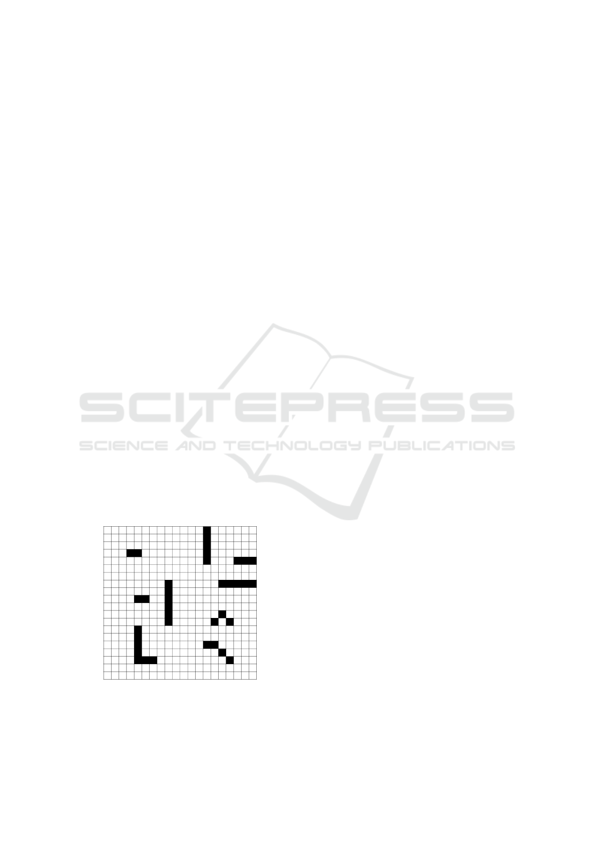
Figure 1: A grid map used in the experiments. Black ver-

tices are impassable obstacles.

The section of 6 by 4 vertices in the top right cor-

ner shall play the role of small but dense part of the

map (Small), while the rest of the grid shall play the

role of large and sparse part of the map (Large). Note

that the graph is connected, so the agents can move

from one part to the other.

The number of agents in the Large part is ﬁxed to

be 10 and the number of agents in the Small part is

increasing by one from 10 to 15. All of the agents

have randomly chosen start and goal locations in their

respective parts of the graph. Each of these settings

was used to create 5 random instances. Together, this

yields 30 instances.

We are also given the information about how to

split the agents into the desired disjoint subsets. No

automatic splitting is implemented at this time.

5.2 Measured Results

The two solvers used are CBS (Sharon et al., 2015)

and reduction of MAPF to SAT via the Picat language

and compiler (version 2.2#3) (Zhou et al., 2015).

Picat is a logic-based multi-paradigm language

that integrates logic programming, functional pro-

gramming, and constraint programming. Most impor-

tantly for our purposes, it contains a SAT compiler

that translates constraints modeled by the Picat lan-

guage into a logic formula in the conjunctive normal

form (CNF) that is in turn solved by the built-in SAT

solver. The main advantage of this approach is the

simplicity of the code, while being comparable with

the state of the art SAT-based MAPF solver (Bart

et al., 2017).

The used cost function is sum of cost since this is

the cost function already available in CBS implemen-

tation. However, it is easy to see that the experiments

can be done with makespan cost function.

All experiments were conducted on a PC with an

Intel

 Core

i7-2600K processor running at 3.40

GHz with 8 GB of RAM.

Given the two subsets of agents A

Small

, A

Large

and

shared graph G, we let both of the solvers compute

instance (G, A

Small

) and (G, A

Large

) with time limit

of 600 seconds. Combination of these solutions is a

solution to the initial instance (G, A). We measured

the computation time for each of the subinstance, let

name them PicatSmall, PicatLarge, CBSSmall, and

CBSLarge.

The times that we are interested in are

Picat = PicatSmall + PicatLarge (9)

CBS = CBSSmall +CBSLarge (10)

Combined = PicatSmall +CBSLarge (11)

The averages of these times for each setting of the

input instances are shown in Figure 2.

Combining Strengths of Optimal Multi-Agent Path Finding Algorithms

229

Figure 2: Experimental results using translation to SAT (via

Picat), CBS algorithm, and combination of both.

We can see that for the instances with fewer

agents, the CBS solver is a clear winner. However,

as the number of agents increase (and thus the Small

part becomes denser), the CBS solver is not able to

ﬁnd a solution within the given time limit.

The computation time PicatSmall increases as

well, but not as rapidly. We can see that the biggest

portion of the computation time Picat is PicatLarge.

These results clearly support our theory that split-

ting the input instance and using different solvers for

each part is beneﬁcial in terms of total computation

time.

6 FUTURE WORK

It is clear that an automatic way of splitting the agents

into independent subsets is needed in order to create a

useful algorithm. To do this, we propose to use Inde-

pendence Detection (ID) algorithm (Standley, 2010).

ID can be used to split an instance into independent

subproblems such that combining their solutions yield

a valid solution for the whole instance. Note that if the

solutions for the independent subproblems are opti-

mal then the combined solution for the whole instance

is also optimal (Standley, 2010).

ID works as shown in Algorithm 1. We start by

assigning each agent into a group and ﬁnding an opti-

mal path for each group. This is a single agent path at

the beginning. We then repeatedly check the solutions

of all groups for conﬂicts. If there is no conﬂict, and

each group has an optimal plan, these plans can be

combined into an optimal plan for the whole instance.

Assume that there are two groups conﬂicting (G

and G

). If we can replan one of the groups while

avoiding conﬂict with the other, and keeping the same

cost of the found plan, we will keep that solution

(lines 9 – 14). If no such replanning is possible, we

have to merge G

and G

into a single new group and

Algorithm 1: Independence Detection.

1: assign each agent to a group

2: compute plan for each group

3: while there is a conﬂict in plans do

4: G

, G

← conﬂicting groups

5: if G

and G

conﬂicted before then

6: merge G

and G

into new group G

7: ﬁnd plan for G

8: continue

9: else if can replan G

and avoid G

then

10: replan G

and avoid G

11: continue

12: else if can replan G

and avoid G

then

13: replan G

and avoid G

14: continue

15: else

16: merge G

and G

into new group G

17: ﬁnd plan for G

18: end if

19: end while

20: solution ← path of all groups combined

ﬁnd a new optimal plan (line 16).

By changing the plan of one group, we can create

a new conﬂict with some other group. This can lead to

inﬁnite cycles. To ﬁx this problem, we have to keep

track of groups that were already checked for con-

ﬂicts. If we visit such a pair again, we are possibly in

a cycle, therefore, we merge the groups immediately

into a new group and ﬁnd optimal paths for that group

(line 5).

There exist some enhancements for ID algorithm

(Standley, 2012). These enhancements include the

way how to prioritize the replanning of the conﬂict-

ing groups, what conﬂict to resolve ﬁrst, and how to

choose the initial path for singe-agent groups (if there

are more possible paths).

Note that ID is independent of the solver used to

compute plans for the groups. We can run both algo-

rithms (CBS solver and Picat solver) simultaneously

each time and use the result of the algorithm that ter-

minates ﬁrst. If it is not possible to run both algo-

rithms in parallel, we can start with either one with

given time limit. If no solution is found in that time,

we run the other algorithm. Again if no solution is

found, we increase the time limit and repeat.

We hypothesize that while the groups are small

(and thus are not dense), CBS solver will outperform

Picat solver. As the groups get bigger (indicating

that there are many conﬂicts among the agents), Pi-

cat solver will outperform CBS solver.

ICAART 2019 - 11th International Conference on Agents and Artiﬁcial Intelligence

230

7 CONCLUSION

In this paper, we studied the problem of multi-agent

path ﬁnding (MAPF), namely, we suggested how

to combine solvers with complementary strengths.

We analyzed two state-of-the-art solvers, CBS and

reduction-based Picat solver, used to solve MAPF op-

timally and for each of them, we identiﬁed what type

of instances are hard for it. We tested this empirically

and observed that dense instances are harder for CBS

algorithm and instances on large graphs are hard for

reduction based algorithms. By manual decomposi-

tion of an example problem, we showed that the pro-

posed combination of solvers indeed improves run-

time signiﬁcantly. As a future (not-yet-implemented)

work, we proposed how to automatically split in-

stances into independent subproblems by using the

Independence Detection algorithm.

ACKNOWLEDGEMENTS

This research is supported by the Czech Science

Foundation under the project 19-02183S any by the

SVV project number 260 453.

REFERENCES

Bart

ak, R., Zhou, N., Stern, R., Boyarski, E., and Surynek,

P. (2017). Modeling and solving the multi-agent

pathﬁnding problem in picat. In 29th IEEE Interna-

tional Conference on Tools with Artiﬁcial Intelligence,

ICTAI 2017, Boston, MA, USA, November 6-8, 2017,

pages 959–966.

Boyarski, E., Felner, A., Stern, R., Sharon, G., Betzalel,

O., Tolpin, D., and Shimony, S. E. (2015). ICBS: the

improved conﬂict-based search algorithm for multi-

agent pathﬁnding. In Proceedings of the Eighth

Annual Symposium on Combinatorial Search, SOCS

2015, 11-13 June 2015, Ein Gedi, the Dead Sea, Is-

rael., pages 223–225.

de Wilde, B., ter Mors, A., and Witteveen, C. (2014). Push

and rotate: a complete multi-agent pathﬁnding algo-

rithm. J. Artif. Intell. Res., 51:443–492.

Kornhauser, D., Miller, G. L., and Spirakis, P. G. (1984).

Coordinating pebble motion on graphs, the diame-

ter of permutation groups, and applications. In 25th

Annual Symposium on Foundations of Computer Sci-

ence, West Palm Beach, Florida, USA, 24-26 October

1984, pages 241–250.

Ryan, M. R. K. (2008). Exploiting subgraph structure

in multi-robot path planning. J. Artif. Intell. Res.,

31:497–542.

Sharon, G., Stern, R., Felner, A., and Sturtevant, N. R.

(2015). Conﬂict-based search for optimal multi-agent

pathﬁnding. Artif. Intell., 219:40–66.

Sharon, G., Stern, R., Goldenberg, M., and Felner, A.

(2011). The increasing cost tree search for optimal

multi-agent pathﬁnding. In IJCAI 2011, Proceedings

of the 22nd International Joint Conference on Arti-

ﬁcial Intelligence, Barcelona, Catalonia, Spain, July

16-22, 2011, pages 662–667.

Silver, D. (2005). Cooperative pathﬁnding. In Proceedings

of the First Artiﬁcial Intelligence and Interactive Digi-

tal Entertainment Conference, June 1-5, 2005, Marina

del Rey, California, USA, pages 117–122.

Standley, T. S. (2010). Finding optimal solutions to coop-

erative pathﬁnding problems. In Proceedings of the

Twenty-Fourth AAAI Conference on Artiﬁcial Intelli-

gence, AAAI 2010, Atlanta, Georgia, USA, July 11-15,

2010.

Standley, T. S. (2012). Independence detection for

multi-agent pathﬁnding problems. In Multiagent

Pathﬁnding, Papers from the 2012 AAAI Workshop,

MAPF@AAAI 2012, Toronto, Ontario, Canada, July

22, 2012.

Standley, T. S. and Korf, R. E. (2011). Complete algorithms

for cooperative pathﬁnding problems. In IJCAI 2011,

Proceedings of the 22nd International Joint Confer-

ence on Artiﬁcial Intelligence, Barcelona, Catalonia,

Spain, July 16-22, 2011, pages 668–673.

Surynek, P. (2010). An optimization variant of multi-robot

path planning is intractable. In Proceedings of the

Twenty-Fourth AAAI Conference on Artiﬁcial Intelli-

gence, AAAI 2010, Atlanta, Georgia, USA, July 11-15,

2010.

Surynek, P. (2014). Compact representations of coopera-

tive path-ﬁnding as SAT based on matchings in bipar-

tite graphs. In 26th IEEE International Conference on

Tools with Artiﬁcial Intelligence, ICTAI 2014, Limas-

sol, Cyprus, November 10-12, 2014, pages 875–882.

Surynek, P., Felner, A., Stern, R., and Boyarski, E. (2016).

Efﬁcient SAT approach to multi-agent path ﬁnding

under the sum of costs objective. In ECAI 2016 -

22nd European Conference on Artiﬁcial Intelligence,

29 August-2 September 2016, The Hague, The Nether-

lands - Including Prestigious Applications of Artiﬁcial

Intelligence (PAIS 2016), pages 810–818.

Yu, J. and LaValle, S. M. (2013). Structure and intractability

of optimal multi-robot path planning on graphs. In

Proceedings of the Twenty-Seventh AAAI Conference

on Artiﬁcial Intelligence, July 14-18, 2013, Bellevue,

Washington, USA.

Zhou, N., Kjellerstrand, H., and Fruhman, J. (2015). Con-

straint Solving and Planning with Picat. Springer

Briefs in Intelligent Systems. Springer.

Combining Strengths of Optimal Multi-Agent Path Finding Algorithms

231