Dynamic Index Tracking via Stochastic Programming

Patrizia Beraldi

, Antonio Violi

1,2

, Maria Elena Bruni

and Gianluca Carrozzino

Department of Mechanical, Energy and Management Engineering, University of Calabria, Rende (CS), Italy

Decision Lab, Mediterranean University of Reggio Calabria (RC), Italy

Keywords:

Index Tracking, Stochastic Programming, Out-of-Sample Analysis.

Abstract:

Index tracking (IT) is an investment strategy aimed at replicating the performance of a given ﬁnancial index,

taken as benchmark, over a given time horizon. This paper deals with the IT problem by proposing a stochastic

programming model where the tracking error is measured by the Conditional Value at Risk (CVaR) measure.

The multistage formulation overcomes the myopic view of the static models considering a longer time horizon

and provides a more ﬂexible paradigm where the initial strategy can be revised to account for changed market

conditions. The proposed formulation presents a bi-objective function, where the two conﬂicting criteria

wealth maximization and risk minimization, are jointly accounted for by properly choosing the weight to

attribute to the two terms. The model is encapsulated within a rolling horizon scheme and solved iteratively

exploiting each time the more update information in the generation of the scenario tree. The preliminary

computational experiments carried out by considering as benchmark the Italian index FSTE-MIB seem to be

promising and show that, on an out-of-sample analysis, the tracking portfolios follow the benchmark very

closely, overcoming it on the long run.

1 INTRODUCTION

Index tracking (IT) is an investment strategy aimed

at replicating the performance of a given ﬁnancial in-

dex taken as benchmark over a given time horizon.

When the portfolio composition mirrors exactly the

index one, i.e. all of the assets that make up the in-

dex are purchased in the same proportion as in the

index, the investment strategy is called “full replica-

tion”. Even though such a strategy would ensure a

perfect match of the index behaviour, the main disad-

vantage is related to the presence of high transaction

costs associated with the purchase and sale of securi-

ties. Indeed, the weights for each asset composing the

index are typically based on market capitalization and

as soon as the prices of the assets change, the weights

are modiﬁed as well. “Partial replication” can be seen

as an alternative approach for index tracking where

only a subset of assets composing the index is prop-

erly selected with the aim of minimizing the tracking

error.

The IT problem has been attracting a growing in-

terest in the scientiﬁc community as witnessed by

the large number of contributions that is sill increas-

ing in the last years. Interested readers are referred,

for example, to (Sant”Anna et al., 2017) for a re-

cent overview on the relevant literature. Most of the

proposed formulations are static models relying on a

backward perspective. The tracking portfolio is built

so to minimize a tracking error that measures the dif-

ference between the historical performance of the de-

ﬁned portfolio and the index. The basic idea is that

higher tracking accuracy in the past is a “guarantee”

for the future. Based on the speciﬁc tracking error

function used, different formulations have been pro-

posed. For example, the variance of the difference be-

tween the benchmark and the tracking portfolios has

been considered in (Corielli and Marcellino, 2006).

The mean absolute deviation (MAD) has been used as

dispersion measure in (Kim et al., 2005) and (Konno

and Yamazaki, 1991), to name a few. The downside

mean deviation, that focuses on the negative side of

the tracking error, appears in (Angelelli et al., 2008),

(Ogryczak and Ruszczy’nski, 1999). Quantile mea-

sures have been used for example in (Ogryczak and

Ruszcz’nski, 2012).

Unlike a backward view, a forward perspective in

static models has been seldom adopted. This new

view changes the nature of the problem, that can not

be considered deterministic any more. Indeed, the

future performance of the index and its components

are not known when the tracking portfolio should

Beraldi, P., Violi, A., Bruni, M. and Carrozzino, G.

Dynamic Index Tracking via Stochastic Programming.

DOI: 10.5220/0007573404430450

In Proceedings of the 8th International Conference on Operations Research and Enterprise Systems (ICORES 2019), pages 443-450

ISBN: 978-989-758-352-0

443

be deﬁned. Following the classical stochastic pro-

gramming framework (Birge and Louveaux, 2013;

Ruszczy

nski and Shapiro, 2003), uncertain parame-

ters can be dealt as random variables deﬁned on a

given probability space and under the assumption of

discrete distribution, they can be represented in terms

of scenarios, each occurring with a given probability

value. A scenario based approach for the IT problem

was proposed by (Consiglio and Zenios, 2001) where

the tracking error is represented in terms of the MAD.

More recently, (Beraldi and Bruni, 2018) addressed

the IT problem by the chance constrained paradigm

(both in the basic and integrated form). Both the back-

ward and the forward perspectives described so far are

deﬁned in a static setting. Once selected, the portfolio

is not rebalanced during the considered time horizon

in the hope that the future behaviour will be close to

the desired one. In a dynamic setting, the portfolio

composition can be revised from time to time accord-

ing to new market information, if the tracking accu-

racy starts to deteriorate. Dynamic index tracking has

been mainly addressed in a deterministic setting. For

example, in (Gaivoronski et al., 2005) the authors pro-

posed several dynamic formulations differing for the

adopted tracking measures. Very recently, Strub and

Baumann addressed in (Strub and Baumann, 2018)

the problem of the optimal construction and rebalanc-

ing of index tracking portfolios. They proposed and

compared different deterministic formulations for re-

balancing that are iteratively solved within a rolling

horizon scheme. A multi-objective evolutionary al-

gorithm has been proposed in (Chiam et al., 2013)

and applied for both the single-period and the multi-

period index tracking problem.

When the dynamic and the stochastic elements are

jointly addressed, the problem becomes even more

challenging. However, only a few number of contri-

butions deal with this more involved case. A two-

stage stochastic programming formulation has been

proposed in (Stoyan and Kwon, 2010). The model

aims at minimizing the MAD risk measure and in-

cludes some real features. The multi-stage paradigm

has been adopted in (Barro and Canestrelli, 2009),

where the authors focus on tracking error measures

and consider as objective function the weighted sum

of a ﬁrst term accounting for the deviation from the

benchmark and a second penalty term accounting for

the portfolio turnover. Local volatility and tail risk are

both controlled in the stochastic formulation proposed

in (Barro et al., 2018).

In this paper, we propose a multistage-stochastic

programming model where tracking accuracy is con-

trolled by the Conditional Value at Risk (Rockafellar

and Uryasev, 2000). While the Value at Risk (VaR)

measures the maximum potential loss that can be ex-

perienced with a given conﬁdence level, the CVaR al-

lows to control the tail risk, determining the expected

value of the losses exceeding the VaR. The relevance

of the CVaR is mainly related to the theoretical prop-

erties it satisﬁes. It is a “coherent” risk measure and

is consistent with the second degree stochastic dom-

inance. From a practical viewpoint, the CVaR is a

downside risk measure in the sense that it does not

penalize the deviations above a given target, typically

perceived as proﬁt. Moreover, the CVaR is appealing

from a computational viewpoint since it admits, in the

case of discrete distributions, a linear programming

reformulation. When the CVaR is embedded within

a multistage model, the problem becomes more difﬁ-

cult to deal with since the time-consistency property

should be properly accounted for. Roughly speaking,

this property asserts that, at every state, optimality of

our decisions should not depend on scenarios that we

already know cannot happen in the future (de Mello

and Pagnoncelli, 2016). Starting from the stage-wise

risk measures properly deﬁned, we build an aggre-

gated measure. It represents the ﬁrst criteria to op-

timize together with the expected wealth. The con-

ﬂicting nature of the two criteria is accounted by con-

sidering a bi-objective function where their relative

importance is weighted by the choice of a parameter

λ between [0, 1].

The rest of the paper is organized as follows. Sec-

tion 2 introduces the multistage stochastic program-

ming formulation. It is embedded into a rolling hori-

zon scheme, as detailed in Section 3. Section 4 reports

on the computational experiments carried out to eval-

uate the performance of the proposed strategy also on

the basis of an out of sample analysis. Conclusions an

future research directions are discussed in Section 5.

2 MODEL FORMULATION

We consider the problem of a fund manager who

wants to determine a portfolio that tracks a benchmark

(market index) over a given time horizon composed

of t ∈ T = {1, . . . , T } discrete time periods. Once ini-

tially composed, the portfolio can be rebalanced (by

buying and/or selling some assets) in response to new

market information.

We denote by {τ

}

t∈T

and {ξ

}

t∈T

, the random

evolution of the market index and the price of the dif-

ferent composing assets. Thus, for every t, ξ

is a

random vector of size |J|, where J denotes the set of

assets. Under the assumption of discrete random vari-

ables, the information structure can be described by

a scenario tree where, at each stage t ∈ T , there is a

ICORES 2019 - 8th International Conference on Operations Research and Enterprise Systems

444

discrete number of nodes N

, referring to a speciﬁc

realization of the uncertain parameters. There are T

levels (stages) in the tree, corresponding to speciﬁc

time periods. The nodes at ﬁnal stage N

are called

leaves. The set N

is composed of a unique node,

i.e. the root. Each node at stage t, except the root,

is connected to a unique node at stage t − 1, which

is called ancestor a(n) and to a set of nodes at stage

t + 1, called successors, denoted by c(n). Leaf nodes

have no successors and identify the scenarios, each

one represented by a path from the root to a leaf, de-

noted P (n). Let π

a(n),n

denote the probability of tran-

sition to node n from its ancestor a(n). The sum of the

probabilities associated to the arcs leaving each node

sum up to 1. Starting from these values, the proba-

bility associated with each node n denoted by p

can

be easily determined as the product of the transition

probabilities. The following notation is used. For

each asset j and node n, let x

, b

and s

denote

the amount of asset j hold, bought and sold at node

n, respectively. Moreover, the possibility of investing

in a riskless asset (liquidity component) that guaran-

tees a given interest, at a rate r

is also considered by

means of variable v

. Portfolio should be composed

and managed in such a way to satisfy the following

set of constraints:

= ¯x

+ b

− s

∀ j ∈ J (1)

= x

ja(n)

+ b

− s

∀ j ∈ J ∀n ∈ N − {0}

(2)

(1 − t

)

∑

j∈J

+C = (1 +t

)

∑

j∈J

+ v

(3)

(1 −t

)

∑

j∈J

+ (1 + r

a(n)

(1 +t

)

∑

j∈J

+ v

∀n ∈ N − {0} (4)

Constraints (1)-(2) are classical balance constraints.

In the case of the root node, ¯x

denotes the initial hold-

ing in asset j, if any. Constraints (3)-(4) are monetary

balance constraints. Here t

denotes the transaction

costs that are assumed to be proportional to the mon-

etary value that is traded. At the initial time, a capital

denoted by C is assumed to be invested. The port-

folio is initially composed and eventually revised in

the subsequent periods with the aim of taking into ac-

count both the expected tracking portfolio value and

the risk, measured in terms CVaR. For a given conﬁ-

dence level α (eventually depending on the stage t),

the CVaR is deﬁned as the expected loss exceeding

the VaR:

IE[L|L ≥ VaR]

In our approach, the loss associated with each node

n of the scenario tree is computed with the respect to

the benchmark, i.e. L

= max(0, K

−W

), where W

represents the value of the tracking portfolio at node n

computed as W

∑

j∈J

and K

is the value

of the initial capital C compounded by considering the

interest rates generated by the market index. Thus,

∏

m∈P (n)−{0}

(1 + τ

) ∗C, where τ

denotes the

rate of return of the market index at nodes m belong-

ing to the path connecting the root with node n. While

in the two stage model, the deﬁnition of the CVaR is

straightforward, in the multiperiod setting it deserves

some additional explanation. To simplify the expo-

sition, we include additional supporting variables de-

noted by CVaR

and CVaRt. For each stage t, the

CVaRt is computed and then the staged values are

properly aggregated. At the second stage, i.e. t = 2,

the CVaRt

can be easily computed by adopting the

classical formula for discrete distributions:

CVaRt

= η +

(1 − α)

∑

n∈N

max(0, L

− η) (5)

where η denotes the VaR and the max(0, L

− η) ac-

counts for the losses exceeding the VaR. This latter

term can be linearized by adding for each node n a

supporting non negative variable δ

≥ L

−η. At later

stages, the CVaRt is determined by considering the

expected risk measures associated with the nodes of

that level, but taking into their “past history”. For ex-

ample for t = 3,

CVaRt

∑

n∈N

∗CVaR

(6)

where for each n, CVaR

is computed by considering

the successors of n and it is deﬁned as

CVaR

= η

(1 − α)

∑

m∈N

|m∈c(n)

max(0, L

−η

(7)

The different stage-wise measures are then aggre-

gated attributing a weight at the different stages (as-

sumed equal in our approach). Although the ultimate

objective is the minimization of the risk component

aimed at controlling the tracking accuracy, the deci-

sion maker is typically also concerned about the max-

imization of the expected wealth accumulated at the

different time periods that may generate an excess of

return over the benchmark. With the aim of taking

both the elements into account, the proposed formu-

lation considers a bi-objective function:

minz = λ (

(T − 1)

∑

t=2

CVaR

) −

(1 − λ)(

(T − 1)

∑

t=2

∑

n∈N

). (8)

Dynamic Index Tracking via Stochastic Programming

445

Here the parameter λ can be interpreted as a risk aver-

sion level as it determines how much weight is given

to minimize risk as opposed to maximize the wealth.

The extreme case of λ = 0 corresponds to the risk neu-

tral case, whereas the higher the λ the greater the im-

portance attributed to risk. The formulation is com-

pleted with the additional supporting variables L

and

used to account for the max operator. Finally, the

model includes a diversiﬁcation constraint that limits

the monetary amount invested in every asset:

≤ θW

∀ j ∈ J, ∀n ∈ N (9)

where θ is a user deﬁned parameter. The overall

model belongs to the class of multistage stochastic

programming linear problems where the non antici-

pativity constraints are implicitly included (node for-

mulation). Depending on the number of time stages

and scenarios the computational effort can become

extremely high calling for the use of solution ap-

proaches exploiting the speciﬁc problem structure.

For the computational experiments presented here-

after the solution time is still affordable by using off-

of-the-shelves software. The design of specialized

methods is the subject of ongoing research.

3 EXPERIMENTAL DESIGN

The proposed formulation is embedded into a rolling

horizon scheme and is solved periodically over the in-

vestment horizon using each time more updated infor-

mation. Even though the use of the rolling approach is

not new in the portfolio optimization context (see, for

example, (Beraldi et al., 2011)), most contributions

for the IT problem consider one period models as in

(Strub and Baumann, 2018). The multistage formula-

tion overcomes the myopic view of these static mod-

els considering a longer time horizon and provides a

more ﬂexible paradigm where the initial strategy can

be revised to account for changed market conditions.

In the proposed experimental design, we consider

a long time horizon starting from a ﬁxed period in the

past denoted by T

and ending at period T

. The plan-

ning horizon is divided into two sets: the ﬁrst set from

to T

is used as “historical source” to determine all

the data required for scenario generation, the second,

lasting at T

is used as investment horizon where the

tracking accuracy is evaluated. The following Figure

1 shows the scheme.

The proposed formulation is solved iteratively

starting from period T

. Once deﬁned the optimal in-

vestment strategy, the decisions referring to the cur-

rent time (ﬁrst stage decisions associated with the root

node of the scenario tree) are implemented. As time

Figure 1: Rolling Horizon process.

progresses, at each subsequent periods the tracking

portfolio can be rebalanced. The multistage model

is solved again using an updated scenario tree rede-

ﬁned using an update set of historical data that also

includes the new information that has been revealed.

The ﬂowchart 2 reported below illustrates the rolling

approach.

Once time index is increased, the parameters

should be updated as follows:

• ¯x

= x

, ∀ j ∈ J

• C = v

(1 + r

4 COMPUTATIONAL RESULTS

This section is devoted to the presentation and dis-

cussion of the computational experiments carried out

with the aim of assessing the performance of the pro-

posed stochastic programming formulation. The im-

plemented code integrates MATLAB R2015b

for the

scenario generation and parameters update phases and

GAMS 24.7.4

as algebraic modeling system, with

CPLEX 12.6.1

as solver for the linear programming

www.mathworks.com

www.gams.com

https://www.ibm.com/analytics/cplex-optimizer

ICORES 2019 - 8th International Conference on Operations Research and Enterprise Systems

446

Figure 2: Flowchart of the rolling approach.

models. All the test cases have been solved on a PC

Intel Core I7 (2.5 GHz) with 8 GB of RAM DDR3.

As benchmark we have considered the FTSE-

MIB

, that is the primary market Index for the Ital-

ian equity markets, capturing approximately 80% of

the domestic market capitalization. FTSE- MIB mea-

sures the performance of 40 Italian equities and seeks

to replicate the broad sector weights of the Italian

stock market.

Moreover, for all the test cases we have considered

a planning horizon of one month with weekly time

stages, an initial cash of e10,000,000, the possibil-

ity to invest in a risk-free asset with an annual return

of 2% and an upper bound to the amount invested in

each asset equal to 5% of the entire portfolio wealth.

As regards the conﬁdence level for the CVaR calcula-

tion we have considered a value of 90%.

Historical data of weekly prices have been col-

lected for the benchmark and the underlying assets

starting from April 2015 to April 2017. Such val-

ues have been used to compute the drift, volatility and

correlation coefﬁcients used to generate the scenario

tree by a Monte Carlo simulation technique assuming

a correlated Brownian motion (Beraldi et al., 2010),

(Beraldi and Bruni, 2013). Each time a scenario tree

https://www.borsaitaliana.it/borsa/indici/indici-in-

continua/dettaglio.html?indexCode=FTSEMIB

is generated within the rolling horizon scheme, more

updated information are used, discarding the oldest

data and adding the new revealed values. The results

reported hereafter refer to a scenario tree with four

stages and 200 scenarios. The designed tree consid-

ers a branching factor decreasing with the time stages.

Several tests have been carried out with the aim of

assessing the performance of the proposed approach

and of gaining managerial insights useful to support

the decision maker in the ﬁnancial planning process.

The ﬁrst set of experiments have been carried out to

evaluate the impact of the risk aversion on the perfor-

mance of the tracking portfolios. The model has been

tested for different values of the parameter λ between

[0, 1]. The results in terms of expected wealth and risk

are shown in Figure 3 that depicts the efﬁcient fron-

tier, i.e. the set of “non-dominated” portfolios.

As expected, a conservative attitude, represented

by a high value of λ, provides less proﬁtable solu-

tions carrying, on the other side, lower risk. A more

aggressive behaviour (low values of λ) leads to the

deﬁnition of portfolios with higher expected wealth

that can be exposed to higher losses. By varying λ,

the decision maker can determine different portfolios

to choose from also according to his/her risk attitude

and contingent market conditions.

Another set of experiments has been devoted to

validate the effectiveness of the proposed approach

in a real-life setting by means of an “out-of-sample”

analysis. We have considered a time horizon of 10

weeks and evaluated the provided solutions on the

data really observed from pril to June 2017. First of

all, we have analyzed the behaviour of solutions ob-

tained with the proposed model (SP) for three differ-

ent values of λ (0, 0.5 and 1) and compared these port-

folios with the benchmark under the independence as-

sumption. The following Figure 4 reports the cumu-

lative returns evaluated over the out of sample hori-

zon. The results clearly show that, irrespective of the

choice of the λ values, the generated portfolios track

very closely the benchmark, overcoming it in the long

run. The best performance seems to be achieved for

a λ value equal to 1, thus when a higher risk aversion

is taken into account. In this case, for all but two pe-

riods, higher cumulative returns are guaranteed when

the investment strategy is applied on real data.

Other experiments have been carried out to evalu-

ate to what extent the rolling approach impacts on the

performance of the investment strategy when tested

on an out of sample analysis. To this aim, we

have compared the results obtained with and without

rolling. In this last case, the initial portfolio obtained

by solving the multistage model and associated with

the root node of the scenario tree is kept for all the

Dynamic Index Tracking via Stochastic Programming

447

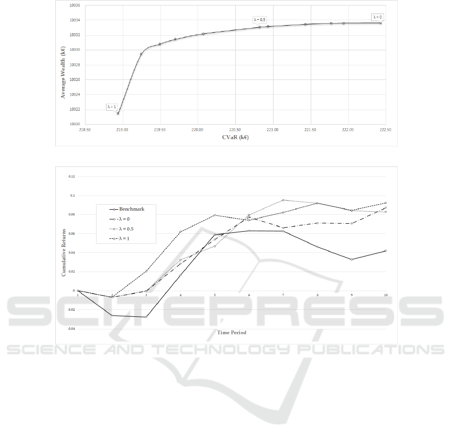
Figure 3: Efﬁcient frontier.

Figure 4: Cumulative returns for the SP portfolios and the benchmark as function of λ.

investment horizon and is not revised any more. The

following Figure 5 reports the cumulative returns ob-

tained for a medium risk-aversion level (λ= 0.5). The

results clearly show the superiority of the rolling ap-

proach that is related to a major ﬂexibility to revise the

portfolio in response to changes in the market condi-

tion. Looking at the Figure, it emerges that, the strate-

gies behave very similarly in the ﬁrst two periods, but

as soon the benchmark modiﬁes its trend, a revision

of the portfolio is required to maintain a high tracking

accuracy.

The better performance of the rolling approach

comes at the price of an increased computational ef-

fort required by the iterated solution of the multistage

problem that is already difﬁcult to solve. A good com-

promise could be to avoid to execute the revision of

the portfolio at regular intervals, but trigger it on the

basis of pre-deﬁned criteria, such large changes of the

market conditions. The deﬁnition of event-triggered

rebalancing would represent a more ﬂexible alterna-

tive to focus on.

5 CONCLUSIONS

The paper deals with the index tracking problem and

proposes a multistage stochastic programming formu-

lation where the tracking accuracy is controlled by the

Conditional Value at Risk measure. With the respect

to the static models, the proposed approach, looking

at a longer horizon and explicitly accounting for un-

certainty, guarantees the deﬁnition of more ﬂexible

investment strategies that could be revised to account

for changed market conditions. A bi-objective func-

tion, merging the two conﬂicting criteria of wealth

maximization and risk minimization, is designed with

the aim of providing the decision maker with different

investment solutions to evaluate by considering differ-

ent levels of risk aversion. The model is encapsulated

within a rolling horizon scheme and solved iteratively

exploiting each time the more update information in

the generation of the scenario tree. The computa-

tional experiments have been carried out by consid-

ering as benchmark the Italian index FSTE-MIB. An

ICORES 2019 - 8th International Conference on Operations Research and Enterprise Systems

448

Figure 5: Cumulative returns with and without the rolling approach for λ = 0.5).

out-of-sample analysis has been performed to evalu-

ate the behaviour of the proposed approach when ap-

plied on a real setting. The preliminary results show

that the tracking portfolios are able to replicate (and

even beat) the benchmark on the long run and em-

phasize the importance of adopting a rolling horizon

approach to guarantee high accuracy levels.

REFERENCES

Angelelli, E., Mansini, R., and Speranza, M. G. (2008). A

comparison of mad and cvar models with real features.

Journal of Banking & Finance, 32(7):1188–1197.

Barro, D. and Canestrelli, E. (2009). Tracking error: A

multistage portfolio model. Annals of Operations Re-

search, 165(1):47–66.

Barro, D., Canestrelli, E., and Consigli, G. (2018). Volatil-

ity versus downside risk: performance protection in

dynamic portfolio strategies. Computational Manage-

ment Science, in press:1–47.

Beraldi, P. and Bruni, M. (2013). A clustering approach for

scenario tree reduction: An application to a stochastic

programming portfolio optimization problem. TOP,

22(3):1–16.

Beraldi, P. and Bruni, M. (2018). Enchanced indiexation via

chance constraints. Technical Report - FERM Labo-

ratory.

Beraldi, P., Simone, F. D., and Violi, A. (2010). Generat-

ing scenario trees: A parallel integrated simulation-

optimization approac. Journal of Computational and

Applied Mathematics, 233(9):2322–2331.

Beraldi, P., Violi, A., and Simone, F. D. (2011). A decision

support system for strategic asset allocation. Decision

Support Systems, 51(3):549–561.

Birge, J. and Louveaux, F. (2013). Introduction to Stochas-

tic Programming. Springer, New York.

Chiam, S., Kan, K., and Mamun, A. A. (2013). Dynamic

index tracking via multi-objective evolutionary algo-

rithm. Applied Soft Computing, 13(7):3392 – 3408.

Consiglio, A. and Zenios, S. A. (2001). Integrated simu-

lation and optimization models for tracking interna-

tional ﬁxed income indices. Mathematical Program-

ming, 89(2):311–339.

Corielli, F. and Marcellino, M. (2006). Factor based

index tracking. Journal of Banking and Finance,

30(8):2215–2233.

de Mello, T. H. and Pagnoncelli, B. K. (2016). Risk aver-

sion in multistage stochastic programming: A model-

ing and algorithmic perspective. European Journal of

Operational Research, 249(1):188 – 199.

Gaivoronski, A. A., Krylov, S., and Wijst, N. V. D. (2005).

Optimal portfolio selection and dynamic benchmark

tracking. European Journal of Operational Research,

163(1):115–131.

Kim, A., Kim, Y. C., and Shin, K. Y. (2005). An algo-

rithm for portfolio optimization problem. Informatica,

16(1):93–106.

Konno, H. and Yamazaki, H. (1991). Mean-absolute de-

viation portfolio optimization model and its applica-

tions to tokyo stock market. Management science,

37(5):519–531.

Ogryczak, W. and Ruszczy’nski, A. (1999). From stochas-

tic dominance to mean-risk models: Semideviations

as risk measures. European Journal of Operational

Research, 116(1):35–50.

Ogryczak, W. and Ruszczy’nski, A. (2012). Dual stochastic

dominance and quantile risk measuress. International

Transactions in Operational Research, 9(5):661–680.

Rockafellar, R. and Uryasev, S. (2000). Optimization of

conditional value-at-risk. Journal of Risk, 2:21–41.

Ruszczy

nski, A. and Shapiro, A. (2003). Stochastic Pro-

gramming, Handbook in Operations Research and

Management Science. Elsevier Science, Amsterdam.

Sant”Anna, L. R., Filomena, T. P., Guedes, P. C., and

Borenstein, D. (2017). Index tracking with controlled

number of assets using a hybrid heuristic combining

Dynamic Index Tracking via Stochastic Programming

449

genetic algorithm and non-linear programming. An-

nals of Operations Research, 258(2):849–867.

Stoyan, S. J. and Kwon, R. H. (2010). A two-stage stochas-

tic mixed-integer programming approach to the in-

dex tracking problem. Optimization and Engineering,

11(2):247–275.

Strub, O. and Baumann, P. (2018). Optimal construction

and rebalancing of index-tracking portfolios. Euro-

pean Journal of Operational Research, 264(1):370 –

387.

ICORES 2019 - 8th International Conference on Operations Research and Enterprise Systems

450