
Machine Learning Approach to the Synthesis of Identification
Procedures for Modern Photon–Сounting Sensors
Viacheslav Antsiperov
Kotelnikov Institute of Radioengineering and Electronics of Russian Academy of Sciences,
Mokhovaya 11-7, Moscow, Russia
Keywords: Photon–Counting Sensors, Target Detection and Identification, Semiclassical Theory of Light Detection,
Poisson Point Process, Machine Learning, EM–Algorithm.
Abstract: The article presents the results of developing a machine learning approach to the problem of object
identification (recognition) in images (data) recorded by photo-counting sensors. Such images are
significantly different from the traditional ones, taken with conventional sensors in the process of time
exposure and spatial averaging of the incident radiation. The result of radiation registration by photo-
counting sensors (image) is rather a continuous stream of data, whose time frame is characterized by a
relatively small number of photocounts. The latter leads to a low signal-to-noise ratio, low contrast and
fuzzy shapes of the objects. For this reason, the well-known methods, designed for traditional image
recognition, are not effective enough in this case and new recognition approaches, oriented to a low-count
images, are required. In this paper we propose such an approach. It is based on the machine learning
paradigm and designed for identifying (low count) objects given by point-sets. Consistently using a discrete
set of coordinates of photocounts rather than a continuous image reconstructed, we formalize the problem in
question as the problem of the best fitting of this set of counts, considered as the realization of a certain
point process, to the statistical description of one of the previously registered point processes, which we call
precedents. It is shown, that applying the Poisson point process model for formalizing the registration
process in photo-counting sensors, it is possible to reduce the problem of object identification to the
problem of maximizing the tested point--set likelihood with respect to the classes of modelling object
distributions up to shape size and position. It is also demonstrated that these procedures can be brought to an
algorithmic realization, analogous in structure to the popular EM algorithms. At the end of the paper we, for
the sake of illustration, present some results of applying the developed algorithms to the identification of
objects in a small artificial data base of low-count images.
1 INTRODUCTION
In recent decades there has been obvious progress in
developing electromagnetic radiation (EMR) sensors
(not only for visible light). The main trend of this
progress – a decrease in the pixel pitch of the
sensors – manifested itself already in the late 1960s
with the creation of CCD cameras. In the early
1990s it was firmly established with the invention of
CMOS solid-state image sensors. In addition to
increasing the spatial resolution of the sensors, this
trend also implies: an increase in the recording rate
as well as in the dynamic range of sensors, their
miniaturization, a reduction in the energy
consumption, etc.
Because of this tendency, when the pitch of the
pixels decreases, the detection of radiation acquires
a more pronounced quantum nature, and in the
limiting case it becomes the detection of individual
photons (photoelectrons). It is a remarkable fact that
this limiting case has already been achieved to some
extent by using several technologies for
manufacturing the so-called photon-counting sensors
(Fossum et al., 2017). As an example, we can point
out electron-multiplying charge-coupled devices
(EMCCD) (Robbins, 2011), single-photon avalanche
diodes (SPAD) (Dutton et al., 2016) and avalanche
photodiodes in Geiger counter mode (GMAPD)
(Aull et al., 2015).
In a sense, such digital photon-counting sensors
can be considered as electronic analogue of classical
photographic plates with their high image quality
standard (Remez et al, 2016). At the same time,
along with the achievement of a high quality
814
Antsiperov, V.
Machine Learning Approach to the Synthesis of Identification Procedures for Modern Photon-Counting Sensors.
DOI: 10.5220/0007579208140821
In Proceedings of the 8th International Conference on Pattern Recognition Applications and Methods (ICPRAM 2019), pages 814-821
ISBN: 978-989-758-351-3
Copyright
c
2019 by SCITEPRESS – Science and Technology Publications, Lda. All rights reserved

comparable with classic images, photon-counting
sensors also have other advantages. Indeed, as at
registration of each photon the released photo-
electron can be immediately transferred into
microprocessor, there is no need to wait until the
sufficient number of electrons is collected to form
the image for a subsequent post-processing. So,
there is no need for a long-time exposure (Chen and
Perona, 2016).
This peculiarity substantially changes the basic
concepts used in the theory and practice of image
processing. For example, in classical applications of
computer vision, the processing of incoming
information is carried out in several steps. In the first
step, a stream of photocounts is accumulated, then,
based on them, the image is restored and in the last
step the image is transferred to specialized
procedures for extracting certain features,
parameters of the objects. On the contrary, when
computer vision is realized with the help of photon-
counting sensors, it is possible, as noted above, to
synchronize the data recording process and the
process of feature extracting directly from the stream
of photocounts. So, in the case of photon-counting
sensors, the need for an intermediate image
reconstruction disappears and a new concept of
“vision without an image” comes into being (Chen
and Perona, 2016)
In this paper, in the context of such a new
concept we present the results of a study in problems
of identification (recognition) of objects (targets)
based on the information obtained directly from the
stream of photocounts. Consistently using a discrete
set of coordinates of photocounts rather than a
continuous image reconstructed, we formalize the
problem in question as the problem of the best fitting
of this set of counts, considered as the realization of
a certain point process, to the statistical description
of one of the previously registered point processes,
which we call precedents. To solve this problem, we
developed an original approach based on the
methods of statistical (machine) learning (Hastie et
al., 2009). In the framework of the proposed
approach, the problem under consideration is treated
as a task of the maximum likelihood matching of test
counts with the probability distribution of counts for
one of the available precedents, which was formed
earlier in the training process. An important
advantage of the proposed approach is that it can be
used to develop effective computational algorithms.
One of such identification algorithms, structurally
similar to the algorithms of the well-known EM
family, is presented in Section 4.
2 STATISTICAL BASES OF
PHOTON-COUNTING
IDENTIFICATION
For the proposed approach to the identification of
objects to be mathematically justified, it is necessary
to formalize the process of registering radiation with
photon-counting sensors. In other words, it is
necessary to choose such a mathematical model, that
most adequately relates the set of registered
photocounts
,
,…,
to the intensity
of
the radiation incident on the sensitive surface Ω of
the sensor. Here the ∈Ω denotes the continuous
coordinates of the point in some coordinate system
in the plane of registration,
are the coordinates of
the pixels corresponding to the registered
photocounts.
In the ideal case, when the size of the pixels can
be considered arbitrarily small − in the so-called
continuous model of the photodetection process
(Goodman, 2015), the coordinates of the counts
are a set of random vectors (of random number ),
even for a given, nonrandom intensity
. The
most general mathematical model for such
phenomenon is a random point process (Streit,
2010). From the semiclassical theory of
photodetection, it is well-known that among such
processes the Poisson point process (PPP) simulates
the mechanisms of photocounts generation in the
most adequate manner (Mandel and Wolf, 1995). A
remarkable feature of PPP is that a complete
statistical description of counts can be determined by
the only function − the count density
− all
finite-dimensional probability distributions of count
coordinates are expressed in terms of it (Streit,
2010):
,
,…,
!
∏
exp
(1)
Quantum theory specifies that the density
in (1)
is related by a simple expression to the intensity
of the incident radiation, namely,
/̅, where is the coefficient of quantum
efficiency of the detector material, is a frame
readout time, ̅ is the central frequency of the
incident radiation and is the Planck constant
(Goodman, 2015).
The above relation, expressing
through
, together with the distributions (1), defines the
model relating the input
of an ideal
(continuous) detector to the statistics of its output −
Machine Learning Approach to the Synthesis of Identification Procedures for Modern Photon-Counting Sensors
815

PPP count coordinates
. For real sensors with
pixels of finite dimensions, the corresponding
relation is obtained by integrating (1) over all pixels,
taking into account the exact numbers of
photocounts
registered by each of them. Note
that the model of the real sensor will be close to the
ideal model (1) in those cases when the probabilities
of two or more photocounts (
1) are small
compared to the probability of one. It is easy to
show that the necessary condition for that is
1, where is the area of an individual
pixel. Thus, when registering weak radiation
→
0, or in high frame rate imaging →0, or in the
case of photon-counting sensors →0, statistical
description (1) is an adequate model for the photon-
counting sensors.
For this reason, the set of finite-dimensional
distributions (1) could be chosen as the basis for the
statistical synthesis of recognition / identification
methods for photon-counting sensors. However, one
more step can be made in this direction if we slightly
extend the formulation of the problem. Namely, let
us take as the identity relation of objects the
similarity of the form of their radiation intensities
regardless of the total brightness of each of them
(see discussion of this formulation in (Antsiperov,
2018.)). From the statistical point of view this
means, that instead of the joint distributions (1) the
conditional distributions of the count coordinates
for a given total number should be chosen as
the basis:
,…,
|
∏
,
.
(2)
The distributions (2) express the known property of
the PPP − the conditional joint distribution of the
counts decomposes into a product of identical
distributions of each of them (Streit, 2010). In other
words, for a given , the counts
are a set of
independent identically distributed (iid) random
vectors. Such samples are the source data for most
statistical approaches, which makes the given
formalization of the problem very attractive.
Moreover, the count distribution
(2) coincides
directly with the (normalized) intensity
and
does not depend on either the detector material , or
the carrier frequency ̅ of the radiation, or the
registration time and pixel area . In view of these
remarkable properties of the distributions (2), they
have a universal character and for this reason they
were chosen as the statistical basis of our approach.
3 PRECEDENT DESCRIPTION
BY GAUSSIAN MIXTURES
As noted in the introduction, the proposed approach
to objects / targets identification is oriented toward
machine learning methods (Hastie et al, 2009).
Therefore, the available precedents are initially also
represented by registered (in the training step) sets
of photocounts, their statistics is also given by
distributions (2). However, the use of the direct
registration data of precedent in identification
procedures is not rational, both because of the low
efficiency of resulting methods, and because of
wasteful use of computing resources (large amounts
of data, respectively, large search times for target
precedents, etc.). The obvious way here is to use the
direct registered data to form some compact
descriptions of precedent radiation intensities
and then to use these descriptions to identify the
tested sets of photocounts.
Any restoration of
from the registered data
is an inverse problem to (2), therefore it belongs
to the class of the so called ill-posed problems. The
standard approach here is to approximate the
intensity, in our case the normalized intensity
,
by model distribution |
, belonging to some
parametric family of distributions with a relatively
small number of parameters
,…,
. A
flexible tool for modelling multivariate distributions
of a rather arbitrary type is a family of Gaussian
mixture models (GMM) (Mengersen, et al, 2011),
that was chosen as the basis for intensity
approximations in the approach under discussion. In
this connection, it is assumed that the intensity of
each (−th) precedent can be approximated by the
sum (mixture) of
two-dimensional Gaussian
(normal) distributions:
|
∑
,
det
,
exp
,
,
,
,
,
,
,
(3)
where parameters
include both the number
of
mixture components and the set of
triples
,
,
,
,
,
, that are probabilities
,
of
belonging count to the component , whose mean
and the matrix of the quadratic form
,
are
respectively
,
and
,
.
The choice of the GMM (3) in addition to the
convenience of modelling / analysis is also
convenient because within the framework of
ICPRAM 2019 - 8th International Conference on Pattern Recognition Applications and Methods
816

machine learning there are effective algorithms to
find maximum likelihood (ML) parameters of the
mixture. The group of such algorithms includes
popular EM-algorithms (Gupta, 2010). For the
version of the EM-algorithm used in our approach in
the training step to form the precedent description,
the number of components
was chosen manually,
other parameters were recursively calculated
according to the following scheme:
Е−step:
for i=1 to n
for j=1 to Nk
,
,
,
,
;
|
1
Σ
,
det
,
exp
1
2
,
;
Σ
,
det
,
exp
1
2
,
;
end;
end;
M−step:
for j=1 to Nk
,
∑
|
,
,
,
∑
|
;
,
,
∑
|
,
,
(4)
end;
4 IDENTIFICATION
PROCEDURE FOR GAUSSIAN
MIXTURES
Having established the form of the precedent
descriptions (3) and the procedure of such
description calculations (4), as a final step in
describing the approach proposed, it is necessary to
define the tested data identification procedure for
these descriptions. The standard step in this direction
is the appropriate choice of a quantitative measure of
correspondence, similarity between the tested PPP
counts
and precedent descriptions from the
generated database (DB). It is reasonable that the
candidate for the role of such a measure of similarity
is, in view of (2) and (3), the (logarithmic)
likelihood function:
ln
∏
|
∗
(5)
where
are the coordinates of the counts of the
PPP tested, and
∗
are the parameters of the –
precedent description, obtained with the help of (4).
Theoretically, calculating measure
for all
–precedents, we could use the maximum likelihood
(ML) approach as the procedure of identification.
Namely, considering
for a given realization
as a function of , we can identify the tested
PPP with the precedent
∗
, which provides the
maximum value for the similarity measure (5):
∗
argmax
(6)
However, from a practical point of view, such an
identification procedure is unrealistic. The problem
here is that in the hypothetical DB the same object
with different locations, scales and foreshortenings
would have different precedent descriptions. The
solution to the problem is the identification of the
tested PPP data
not with a specific precedent
description, but with a whole class of similar
descriptions, each of which is obtained from the
single one by some group of transformations. For
example, if we restrict ourselves to the group of
affine transformations →
⁄
(translate to
vector
and scale in times) and give some a priori
distribution
,, then identification can still be
carried out on the basis of the ML approach (6), but
as a measure of similarity we should use
–
the logarithm of the averaging over
, of all
descriptions
|
∗
, obtained from
|
∗
by the group actions:
ln
,
∏
,
,
(7)
,
|
∗
∑
,
∗
det
,
∗
exp
,
∗
.
Using the definition (7) and utilizing the variational
Bayesian approach, we have synthesized the
following EM-like algorithm (Antsiperov, 2019) for
calculating the identification procedure similarity
measure
(7):
Е−step:
for i=1 to n
for j=1 to Nk
Machine Learning Approach to the Synthesis of Identification Procedures for Modern Photon-Counting Sensors
817

,
̅
,
∗
,
∗
̅
,
∗
;
|
,
∗
det
,
∗
exp
,
Σ
∑
,
∗
det
,
∗
exp
,
;
;
end;
end;
M−step:
for j=1 to Nk
∑
|
;
∑
|
;
∑
|
;
(8)
σ
2
∑
,
∗
;
∗
,
∗
;
∗
,
∗
,
∗
;
where
∗
,
∗
;
Σ
∑
,
∗
,
∗
,
∗
∑
,
∗
;
∑
,
∗
;
;
;
̅
;
̅
;
end;
Note that the essence of the synthesized
algorithm (8) is that it recursively calculates the ML
values
∗
and
∗
of the parameters
and , which
specify the most likelihood fitting of the registered
for the description
∗
,
̅
∗
(7) from the
class defined by the description of
|
∗
(3).
Correspondingly, it can be shown that for some
natural assumptions (see (Antsiperov, 2019)) the
similarity measure
(7) converges
to
(5) with the parameters
,
∗∗
,
∗
∗
/
̅
∗
and
,
∗∗
̅
∗
,
∗
:
ln
∗
,
̅
∗
≅
≅
(9)
5 SIMPLE EXPERIMENTS ON
IDENTIFICATION OF
OBJECTS ON ARTIFICIAL
IMAGES
In this paper, for the purpose of illustrating the
proposed identification method, the results of a
computational experiment for a small, artificially
formed database are presented. Descriptions of
precedents in this database were obtained in
processing registration data of the objects with the
simple structure. The latter are chosen as binary
images from the well-known base “MPEG-7 Core
Experiment CE-Shape-1” (Latecki et al., 2000). This
image base is usually used to compare the shape
recognition algorithms and includes 70 categories of
objects with 20 images in each category.
From the MPEG-7 database were arbitrarily
chosen as precedents images of 5 different
categories - “device1-7”, “device5-16”, “heart-14”,
“shoe-8”, “turtle-9”. For unification, they were
reduced to a size of 500 × 500 pixels and centred in
the frames. Since the form of the object’s intensity is
simple - uniform over the object, the simulation of
registration data of precedents was trivial – 1000 of
the first uniformly distributed across the frame
random points that fell into the object were selected.
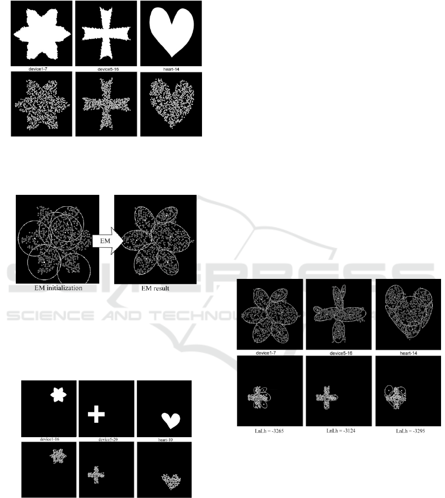
The example of the precedent object and
corresponding registration data (1000 samples) are
presented in Figure 1.
To form a description of the selected precedents
in the form of Gaussian mixtures with
6
components (for all precedents), the EM-algorithm
discussed above, in Section 3, was applied. Figure 2
shows the results of initialization and application of
the EM-algorithm for the formation of the “device1-
7” precedent description (see Figure 1). The
components of the initial and resulting description
are represented by centres and ellipses of constant
ICPRAM 2019 - 8th International Conference on Pattern Recognition Applications and Methods
818
level ~
from the absolute maximum of the entire
Gaussian mixture.
Figure 1: Precedents from the “MPEG-7” database
(Latecki et al., 2000) represented by 500 × 500 binary
images (top) and their registration model data as 1000
samples, uniformly distributed over their shapes (bottom).
Figure 2: The results of initialization (on the left) and the
application (on the right) of the EM – algorithm for the
formation of the “device1-7” precedent description. The
components of the corresponding mixtures are represented
by their centres (points) and lines (ellipses) of a constant
level, approximately 0.1 times the maximum value of the
entire distribution.
Figure 3: The tested objects from the database “MPEG-7”
(Latecki et al, 2000) are selected from the same categories
as the precedents in Figure 1 but shifted and reduced
randomly (top) and model data of their registration in the
form of uniformly distributed 300 counts (bottom).
As the tested objects, the images “device1-16”,
“device5-20”, “heart-10”, “shoe-11”, “turtle-7” were
selected from the same 5 categories as the
precedents. All of them were reduced to the same
size of 300 × 300 points (with the scale = 0.6) and
randomly disposed from the centre of the frames 800
× 800. The simulation of registration data was a
selection of 300 generated random points, uniformly
distributed within the shapes of the objects. Tested
objects and the corresponding registration data (300
samples) are presented in Figure 3.
For each of the tested objects an array of
similarity measure values was calculated for each of
the precedent. Essentially, as noted above, the
similarity measures calculated on the basis of the
proposed procedure are (logarithmic) likelihood
functions
(9) assuming that
are the
result of registering the samples of the –precedent
affine transformation with maximum likelihood
parameters
∗
and
∗
(8). Recalculated with
∗
and
∗
(their own for each precedent) descriptions
, (7) for “device1-7”, “device5-16”,
“heart-14” and the values of the corresponding
LnLf (9) for the registration data of the
tested object “device5-20” are presented in Figure 4.
The full results of the calculation based on the
proposed identification procedure, including all
tested objects are presented in Table 1.
Figure 4: Descriptions of precedents from the database
(top) and their recalculated using the found maximum-
likelihood parameters
∗
and
∗
(8) descriptions
(bottom) for the registration data of the tested object
“device5-16” (see Figure 3). Below for each precedent the
logarithm of the mean likelihoods denoted as “lnLh” are
represented.
Note that the identification based on the criterion
(6) for the set of all precedents (categories) in all
cases of tested objects (in rows of Table 1) is
correct. By the way, there is no such regularity
among the values of the log-likelihood function for a
Machine Learning Approach to the Synthesis of Identification Procedures for Modern Photon-Counting Sensors
819

given precedent. For example, in the case of
precedent “heart-14” (in the corresponding column
of Table 1), the probabilities of data for objects
“device1-16”, “shoe-11”, “turtle-7” are higher than
the probability of data for an object “heart-10” of
the same category as the precedent. However, in the
remaining columns, the expected behavior still
occurs. The marked asymmetries can be related to
the inequality of data volumes for precedents (1000)
and for the tested objects (300).
Table 1: Values of the similarity measure (log likelihood)
for tested objects of different categories (300 samples
data).
Tested
objects
Precedents
device1-7 device5-16 heart-14 shoe-8 turtle-9
device1-16 -3153 -3458 -3228 -3296 -3287
device5-20 -3265 -3124 -3295 -3381 -3271
hear
t
-10 -3362 -3451 -3250 -3437 -3332
shoe-11 -3231 -3272 -3199 -3024 -3246
turtle-7 -3173 -3330 -3165 -3242 -3062
Of course, for an objective, statistically reliable
assessment of the proposed approach, it is necessary
to test it on much larger databases, however, the
results obtained already suggest optimistic
predictions regarding its potential.
6 CONCLUSIONS
It is shown in the paper, that the formalization of the
process of registering radiation by photon-counting
sensors by the model of Poisson point processes
(Streit, 2010) is most adequate from the physical
(quantum) point of view (Goodman, 2015) and
extremely fruitful for the statistical approaches
(Hastie, et al, 2009). On this basis, using the
principles of machine learning (Mengersen, et al,
2011), we succeeded in developing an effective
approach to the synthesis of procedures for
identification (recognition) of objects belonging to a
well-proven family of EM-algorithms. Numerical
simulation (Antsiperov, 2019) showed that the
synthesized identification procedure has a high
convergence rate: for the complexity of describing
precedents of Gaussian mixtures with
~10
components recursive calculations (8), converge in
less than 10 iterations.
ACKNOWLEDGEMENTS
The author is grateful to the Russian Foundation for
Basic Research (RFBR), grant N 18-07-01295 for
the financial support of this work.
REFERENCES
Fossum, E. R., Teranishi, N., Theuwissen, A., Stoppa, D.,
Charbon, E., Eds., 2017. Photon–Counting Image
Sensors. MDPI Books under CC BY–NC–ND license.
Robbins, M., 2011. Electron-Multiplying Charge Coupled
Devices-EMCCDs. In Single-Photon Imaging, P. Seitz
and A. J. P. Theuwissen Eds., Berlin, Springer, pp.
103-121.
Dutton, N. A. W., Gyongy, I., Parmesan, L., Gnecchi, S.,
Calder, N., et al, 2016. A SPAD–based QVGA image
sensor for single–photon counting and quanta imaging.
In IEEE Trans. Electron Devices, vol. 63, no. 1, pp.
189-196, January.
Aull, B. F., Schuette, D.R., Young, D.J., Craig, D.M.,
Felton, B.J., Warner, K., 2015. A study of crosstalk in
a 256x256 photon counting imager based on silicon
Geiger–mode avalanche photodiodes. In IEEE Sens.
J., vol. 15, no. 4, pp. 2123-2132.
Remez, T., Litany, O., Bronstein, A., 2016. A picture is
worth a billion bits: Real–time image reconstruction
from dense binary threshold pixels. In Proceedings of
the 2016 IEEE International Conference on
Computational Photography (ICCP), Evanston: IL,
USA, pp. 1-9.
Chen, B., Perona, P., 2016. Vision without the Image. In J.
Sensors, vol. 16, no. 4, pp. 484.
Hastie, T., Tibshirani, R., Friedman, J., 2009. The
Elements of Statistical Learning. 2
nd
edition, New
York, Springer.
Goodman, J.W., 2015. Statistical Optics, 2
nd
edition. New
York, Wiley.
Streit, R. L., 2010. Poisson Point Processes. Imaging,
Tracking and Sensing. New York, Springer.
Mandel, L., Wolf, E., 1995. Optical Coherence and
Quantum Optics. Cambridge, Cambridge University
Press.
Antsiperov, V., 2018. Precedent–based Low Count Rate
Image Intensity Estimation using Maximum
Likelihood Distribution Descriptions. In Proceedings
of the International Conference on Pattern
Recognition and Artificial Intelligence, Montreal: 13-
17 May, pp. 707–711.
Mengersen, K. L., Robert, C. P., Titterington, D. M., Eds.,
2011. Mixtures: Estimation and Applications, 1st ed. //
John Wiley & Sons.
Gupta, M. R., 2010. Theory and Use of the EM Algorithm.
In Foundations and Trends in Signal Processing, vol.
1, no. 3, pp. 223-296.
Antsiperov, V., 2019. Identification of objects on low–
count images using maximum–likelihood descriptors
ICPRAM 2019 - 8th International Conference on Pattern Recognition Applications and Methods
820

of precedents. In J. Pat. Recogn. and Image Anal.,
Vol. 29, No. 1, (to be printed).
Latecki, L. J., Lakmper R., Eckhardt U., 2000. Shape
Descriptors for Non-rigid Shapes with a Single Closed
Contour. In Proc. IEEE Conf. Computer Vision and
Pattern Recognition, pp. 424–429.
Machine Learning Approach to the Synthesis of Identification Procedures for Modern Photon-Counting Sensors
821
