
Modeling Approaches for Controller Design using the Example of a
Valve-driven Force-controlled Bearing Preload Element
Georg Ivanov, Christian Rutter, Thomas Reuter and Thomas Burkhardt
ICM – Institut Chemnitzer Maschinen- und Anlagenbau e.V., Otto-Schmerbach-Str. 19, Chemnitz, Germany
Keywords: System Simulation, Modeling Approaches, Controller Development, Bearing Preload, CNC-Spindle.
Abstract: Conventional machine tool spindles are factory-equipped with a fixed bearing preload. Depending on the
preload level, the field of application of a machine tool is limited to certain processing tasks. As part of a
collaborative project between ICM e.V., Spindel- und Lagerungstechnik Fraureuth GmbH and SITEC
Automation GmbH, funded by the European funding initiative EFRE, a novel adaptronic machine tool
spindle has been developed. The new spindle offers the possibility of a variable adjustment of the bearing
preload, whereby the machining spectrum of the machine tool can be significantly expanded. The functional
principle is a rotationally symmetrical hydraulic bearing preload element integrated in the main spindle. By
changing the pressure in the oil filled preload element, a relative displacement of the bearing rings is caused.
The bearing preload can be varied proportionally to the relative bearing stroke. Aim of the investigation was
to compare different levels of detail in modeling the main system components and the overall control
system for the purpose of controller development. Therefor the Modelica-based simulation environment
SimulationX® was used.
1 INTRODUCTION
Figure 1 shows an adaptronic main spindle for CNC
lathes developed at ICM e.V. The stepless
adjustment of the bearing preload takes place
according to (Ivanov, 2018) via a rotationally
symmetrical preload element integrated between
housing and spindle shaft.
Figure 1: Structure and functional principle of the
adaptronic main spindle developed at ICM e.V., based on
(Ivanov, 2018).
By varying the oil pressure, a deformation of the
preload element membrane is caused. The stroke of
the preload element thus produced is transmitted on
the outer ring of the rear roller bearing via a Z-
bushing. The relative displacement between inner
and outer ring causes an axial bracing on the
bearings. The preload force can therefore be
controlled via the stroke of the preload element.
Core of the current investigation was the
comparison of different modeling approaches for
mapping control loop components and the overall
control loop in a system simulation environment.
The aim was to investigate how different modeling
approaches of the main components and the overall
control system affect the model accuracy, in
particular the closed-loop behavior, and the
simulation performance.
2 MODELING APPROACHES
FOR 4/3-WAY CONTROL
VALVES
Three control valve models have been compared
with measured data according to their model
accuracy. The investigation included an analytical
Ivanov, G., Rutter, C., Reuter, T. and Burkhardt, T.
Modeling Approaches for Controller Design using the Example of a Valve-driven Force-controlled Bearing Preload Element.
DOI: 10.5220/0007685101890196
In Proceedings of the 9th International Conference on Simulation and Modeling Methodologies, Technologies and Applications (SIMULTECH 2019), pages 189-196
ISBN: 978-989-758-381-0
Copyright
c
2019 by SCITEPRESS – Science and Technology Publications, Lda. All rights reserved
189

model based on the flow-load-function according to
(Weber, 2011), a model based on the measured 3D-
flow-maps of the different control edges and an
analytical model from the model library of the used
simulation program (SimulationX®).
2.1 Flow-load Model
The transmission behavior of the control valve can
be subdivided into its dynamic (valve spool
movement) and its static (flow behavior)
transmission behavior. The temporal course of the
spool position can be described according to
(Weber, 2011) by a second order differential
equation (PT2 element):
(1)
is the characteristic frequency of the undamped
oscillation of the control valve, the damping ratio
and
the valve gain. The solution of the
differential equation gives the temporal course of the
spool position as a function of the control valve
voltage. The flow behavior of the control valve can
be described in simplified terms with the flow-load
function according to (Weber, 2011). For an
application-specific description of the flow behavior
when the consumer port B is blocked, the
description of the two control edges P-A and A-T is
sufficient:
(2)
(3)
Therefor
designates the system pressure before
the control valve,
the pressure at the consumer
connection A, the current spool position and
the maximum spool position. The two constants
and
take into account the different
overlap ratios of the control edges. The nominal
volume flow
and the nominal pressure
have been determined metrologically. The volume
flow at the consumer connection of the control valve
results from the difference between the two control
edge flows:
(4)
2.2 Measurement based
3D-Map-model
The mapping of the dynamic transfer behavior is
equivalent to the analytical model. The static
transmission behavior is realized by implementing
the experimentally determined 3D-flow-maps of the
two control edges P-A and A-T in the model. The
3D-flow-maps match the following form:
(5)
(6)
The volume flow at the consumer connection is
calculated according to equation (4). For a realistic
application-specific mapping of the control valve, its
flow behavior in the small signal range (between -1
to 1 V) is particularly important. Background is the
high pressure gain of the control valve.
2.3 SimulationX-model
The mapping of the dynamic transmission behavior
is analogous to the analytical model described
above. The control valve model of the used
simulation software (SimulationX®) is based on the
orifice formula - see for example (Hatami, 2013).
(7)
For each control edge of the control valve, the flow
is calculated separately. The maximum flow cross
sections of the control edges are calculated on the
basis of simplifying assumptions from the
metrologically determined nominal flow rate, the
nominal pressure and the oil density during the
experimental investigation of the valve.
(8)
For calculating the flow coefficient , a case
differentiation between laminar and turbulent flow
takes place:
(9)
Here
marks the critical Reynolds number and
a constant value for the flow coefficient in the
turbulent range. The Reynolds number is
calculated from the current volume flow over the
respective control edge, the hydraulic diameter
,
SIMULTECH 2019 - 9th International Conference on Simulation and Modeling Methodologies, Technologies and Applications
190
the flow cross section of the control edge and the
kinematic oil viscosity .
(10)
For calculating the hydraulic diameter, a circular
geometry of the flow cross section of the control
edges is assumed.
(11)
The calculation of the pressure loss factor is based
on the equation for sharp-edged circular orifices
given by (Töpfer and Schwarz, 1988):
(12)
The determination of the contraction coefficient
also takes place according to (Töpfer and Schwarz,
1988) via an empirical formula:
(13)
2.4 Comparison of Modeling
Approaches for Control Valves
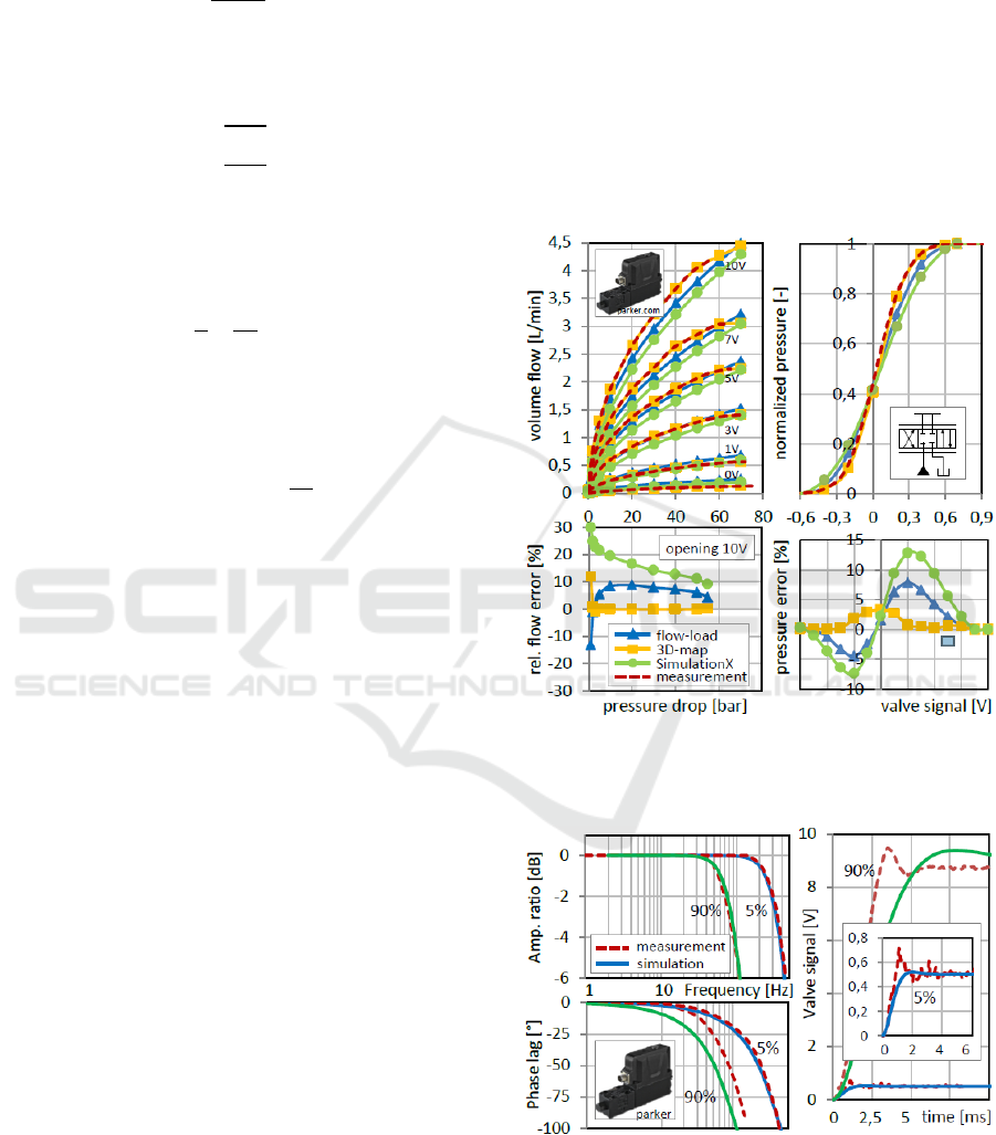
Figure 2 shows a comparison of the simulation
results of the three control valve models with the
results of the metrological characterization of the
control valve. The highest accuracy can be achieved
with the measurement based 3D-map-model. The
model inaccuracy is - except very low pressures -
less than 5 % in the entire operating range. Therefor
the flow pressure drop characteristic (left, control
edge P-A) and the pressure gain characteristic (right)
of the different valve models have been compared to
the measured data.
With the analytical model based on the flow-load
function, model accuracies of up to 95% can be
achieved. The lowest model accuracy is provided by
the SimulationX®-own valve model. The
disadvantage of the flow-load-model and the 3D-
map-model, however, is that no dependence of the
transfer behavior on the oil viscosity and the
temperature can be represented. These models are
only valid for certain temperature conditions of the
hydraulic system, while the SimulationX model
takes the viscosity dependence of the flow behavior
into account.
Figure 3 shows a comparison of simulated and
metrologically recorded frequency responses and
step responses of the control valve. The dynamic
valve behavior, especially in the interesting small
signal range, can be mapped very well by a PT2
element. Amplitude ratio and phase lag can be
reproduced realistically in the complete frequency
range for small input signals. For larger input
signals, the model lags behind the real valve. This is
also confirmed by the comparison of the model step
responses with the measured data. For the controller
design, the small signal range is of superior
importance. For the parameterization of the models
the characteristic frequency and the damping ratio of
the small value range should be used.
Figure 2: Comparison of the static transmission behavior
of different control valve models with measurement
results.
Figure 3: Comparison of the dynamic transmission
behavior of control valve models with measurement
results, left: frequency responses, right: step responses.
Modeling Approaches for Controller Design using the Example of a Valve-driven Force-controlled Bearing Preload Element
191
3 MODELING OF PRELOAD
ELEMENT AND
SPINDLE-BEARING SYSTEM
For the overall mapping of the controlled system, the
valve driven hydraulic bearing preload element and
the spindle bearing system are to be modeled. The
preload element can be described according to
(Ivanov, 2018) as a coupling of plunger cylinder and
spring-damper element. The spring stiffness of the
preload element was determined experimentally.
The effective piston area of the element was
assumed to be constant and generated from the CAD
data. The transfer behavior of the preload element
can be described, by disregarding the element
membrane mass:
(14)
The spring stiffness is in multi-dimensional
dependence on the preload element stroke and the
acting load force (the acting preload force). The
damping was assumed to be constant and has been
estimated.
(15)
The spring force dependence on stroke and load of
the preload element could be determined
experimentally and can be described by an
approximation function of the following form:
(16)
The spindle-bearing system can be described
according to (Ivanov, 2018) by linked spring-damper
elements. The axial stiffness-stroke curves of the
rolling bearing models used in the prototype were
calculated on the basis of a theoretical model
according to (Harris, 2001) and then compared with
experimental results. To describe the transmission
behavior of the spindle-bearing system, the
following equation can be used taking into account
the spindle inertia.
(17)
Therefor
is the total stiffness and
is the total
damping of the spindle-bearing system. The axial
spring force curves of the individual rolling bearings
can be described regarding to (Harris, 2001) by third
degree polynomials:
(18)
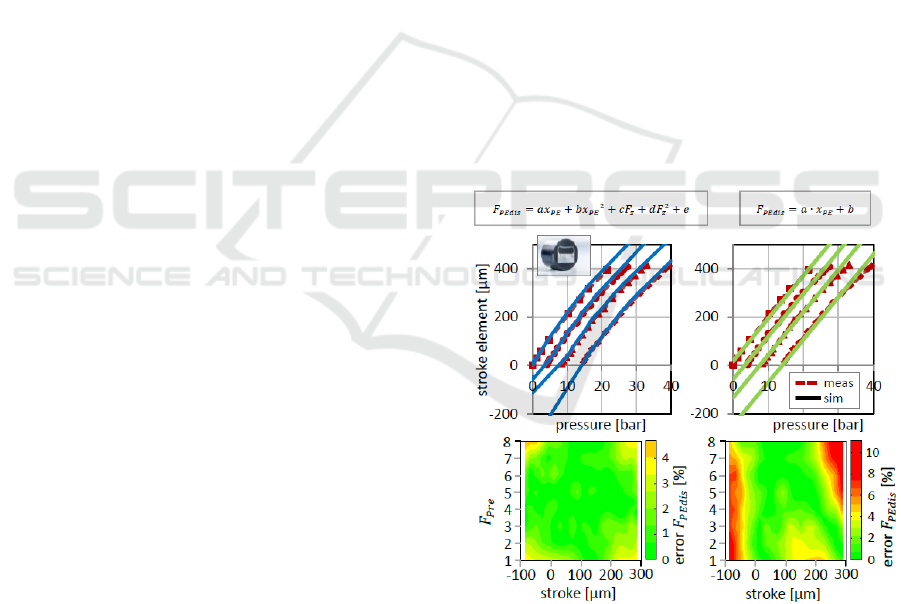
Figure 4 shows a comparison of measurement and
simulation results of the preload element. The
experimentally determined stiffness characteristic of
the preload element was approximated by a three-
dimensional approximation function (left) and by a
simple linear function (right). Figure 4 - below -
shows the relative errors between the measured and
approximated spring force characteristics of the
preload element. With the multi-dimensional
approximation function, a very high agreement with
the measurement results can be achieved. The
maximum relative error in the considered value
range is less than 5%. By approximating the spring
force characteristic by means of a simple linear
function also very high matches can be achieved in a
wide value range. With negative strokes
(compression of the preload element) and very large
strokes the accuracy decreases progressively.
Both approximation functions were used to
parameterize the simulation model. Figure 4 - top -
shows a comparison of the simulation results of the
differently parameterized models with measurement
results. In the experiment the pressure in the element
was increased while a constant external load force
was acting. Thereby the preload element pressure,
the stroke and the load force have been measured. It
could be shown that – in the interesting value range
– the model accuracy cannot be significantly
improved by the application of a multi-dimensional
approximation function.
Figure 4: Comparison of measurement and simulation
results (top) and the spring force of the preload element
(bottom), left: three-dimensional approximation function,
right: linear function.
The comparison of measurement and simulation
results of the axial spring force curves of the
individual spindle bearings shows significant
SIMULTECH 2019 - 9th International Conference on Simulation and Modeling Methodologies, Technologies and Applications
192
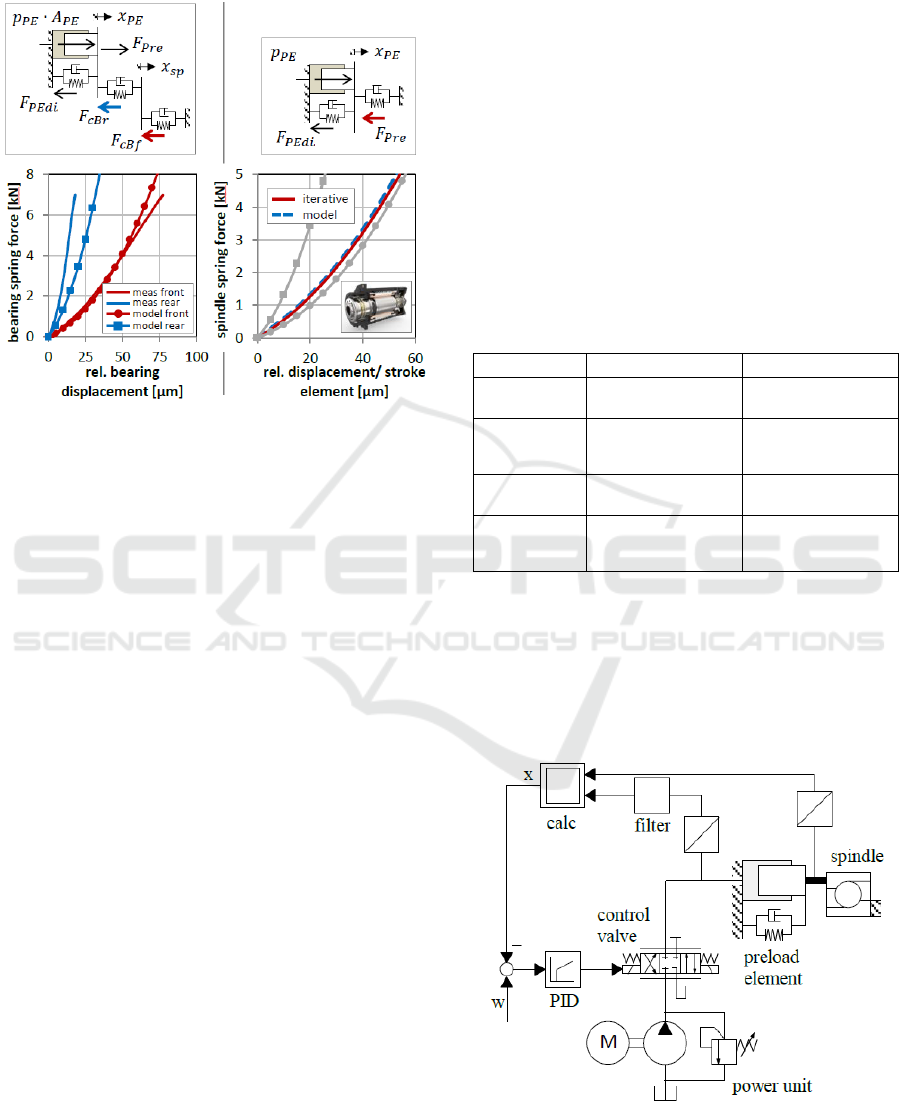
deviations – see Figure 5, left. These are due to the
applied indirect measurement method.
Figure 5: Left - comparison of bearing force curves from
measurement and theoretical calculation model (Ivanov,
2018), right - comparison of spindle force curve from
iterative calculation and SimulationX model.
Since no force measurement is provided in the
prototype spindle, the axial bearing spring forces
had to be calculated indirectly from the measured
preload element stroke, the measured spindle stroke
and the preload element pressure using equation
(15). The resulting inaccuracies lead to the strong
deviations to the calculated bearing spring force
curves. A more accurate measurement of the spindle
bearings should be made on the single bearing with
direct force measurement. To parameterize the detail
model presented in chapter 4, the results of the
theoretical calculation model have been used. The
axial bearing damping was assumed to be constant
according to (Backhaus, 2008).
Figure 5 - right shows the determined total spring
force curve of the spindle. The spindle force curve
was at first generated on the basis of a simplified
iterative calculation and secondly by using the
SimulationX model parameterized with the bearing
force curves. The material stiffness of the spindle
shaft itself was neglected. In the range of interest,
only slight deviations between the two approaches
can be observed. For the parameter-ization of the
signal flow model presented in point 4, the
iteratively determined curve was used.
4 CONTROL LOOP MODELING
APPROACHES
For the design of an optimal force controller, two
simulation models of the control loop have been
developed on the basis of the previously given
analytical descriptions, a detailed physical
simulation model a) and a simplified signal flow
model b) - see Figure 5. The parameterization of the
physical detail model was based on two-dimensional
curves, three-dimensional maps and approximation
functions which were calculated from the
experimentally determined data of the three main
components.
Table 1: Parameterization differences between detail
model and simplified signal model.
parameter
detail model
signal model
pressure
supply
pump with pressure
relief valve
constant pressure
default
control valve
static
3D-maps for control
edges
P-A and A-T
flow-load-function
force preload
element
3D-approx-imation
function
linear function
force of
spindle
bearings
single bearing spring
forces
resulting spindle
spring force
The parameterization of the signal flow model
was based on the analytical flow-load function for
the description of the control valve and simplified
approximation functions for mapping the preload
element and the spindle-bearing system. Important
parameterization differences of the two models are
summarized in Table 1.
Figure 6: Structure of physical detail model.
Modeling Approaches for Controller Design using the Example of a Valve-driven Force-controlled Bearing Preload Element
193
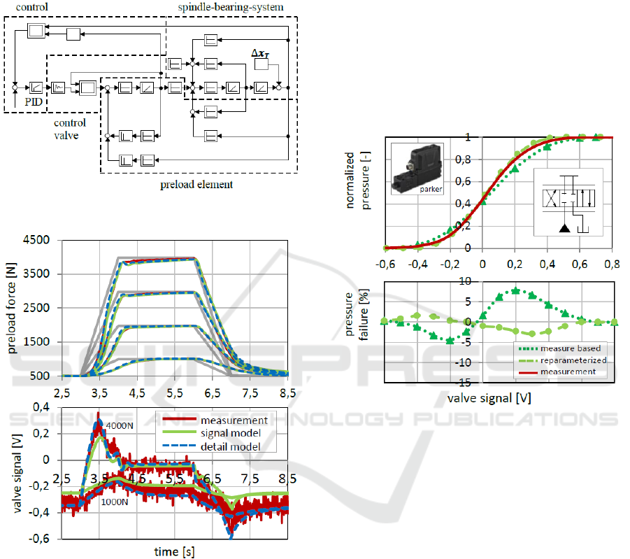
Figure 6 shows the basic structure of the
physical control system and the developed detailed
simulation model and Figure 7 the structure of the
simplified signal flow model of the control system.
Figure 7: Structure of simplified signal flow model.
Figure 8: Validation and comparison of simulation
accuracy of the detail model and the simplified signal flow
model.
Figure 8 shows a comparison of simulation and
measurement results for ramp-shaped control inputs.
The parameterization of the PID controller took
place through systematic trial and error in the
experiment.
The control variable and the valve control signal
curves show that a high degree of conformity of the
detail model with the real system could be achieved.
The simulation results of the simplified signal flow
model show minor static deviations. To increase the
signal model accuracy, the parameterization of the
control valve model had to be adapted. Figure 9
shows the approximation of the pressure-signal
curve to the experimentally determined curve by
shifting the control edge ratios of the flow-load
valve model.
The experimentally determined negative control
edge coverage of 0.6 V for P to A and 0.7 V for A to
T were set to 0.45 V and 0.5 V. The reparameter-
ization leads to a significantly higher model
accuracy with respect to the controlled variable
curves, but to slightly higher deviations of the
control signal curves of the simplified model.
Figure 9: Reparameterization of the flow-load valve model
for increasing the signal flow model accuracy.
5 PERFORMANCE
COMPARISON
Figure 10 shows a comparison of the simulation
time of the detailed model and the simplified signal
flow model. It was shown that the calculation time
can be reduced by at least 75 % compared to the
detailed model by using the signal flow model.
Background is the lower number of state variables to
be calculated as well as the significantly reduced
parameterization of the signal flow model.
The significantly lower simulation time of the
signal flow model becomes especially important
when performing variant simulations, for example
for parameter optimizations. An external parameter
optimization function was used to optimize the
linear PID controller. To investigate the potential of
the shown modeling approaches for parameter
optimizations the function has been applied to both
SIMULTECH 2019 - 9th International Conference on Simulation and Modeling Methodologies, Technologies and Applications
194
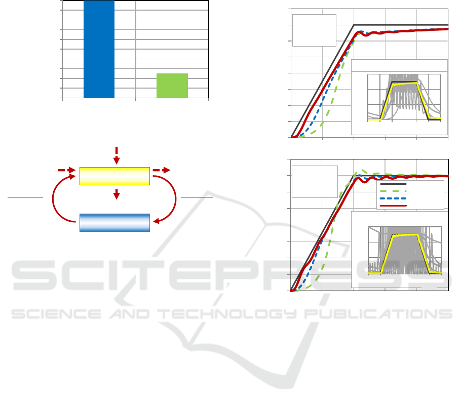
models. The software concept of the developed
optimization function is shown in Figure 11.
Figure 10: Comparison of simulation time.
Figure 11: Software concept of the external optimization
function, based on (Lohse, 2015).
The simulation program (SimulationX®) is
controlled via an existing COM interface by the
optimization function of the external program. The
function loads the corresponding simulation model
and commits the parameters to be optimized - the
parameters of the PID controller. After completion
of the simulation, the time profiles of the control
input (setpoint value) and the control variable (actual
value) are transferred to the optimization function.
The automated evaluation of the control quality
takes place within the optimization function by a
modified ISE criterion according to (Lohse, 2015).
Thereby is the control deviation and its time
derivative.
(19)
Figure 12 shows the results of the external controller
optimization. A robust PID control was designed. A
robust control must always be designed at the most
unfavorable operating point of the control system.
When the main spindle is heavily loaded, the
temperature of the spindle shaft and housing
increases. It is assumed that a relative thermal
expansion of the spindle shaft relative to the housing
of maximum 400 µm can take place. Since the
oscillation susceptibility of the control loop
increases with increasing thermal expansion, the
robust control must be designed for a maximally
stretched spindle.
Figure 12: Performance comparison of detail and signal
flow model by applying an external parameter
optimization function for controller optimization.
For a maximally defined calculation time of both
optimization runs, a distinctly coarser interval
nesting was used in the application of the detail
model, since the calculation time of the detail model
for a single simulation run is approximately 4 times
higher than that of the signal flow model. The result
is a much greater optimization potential of the
controller when using the simplified signal flow
model. The controller parameterization determined
with the signal flow model was tested in the detailed
model and led to almost identical simulations
results.
6 CONCLUSIONS
The presented investigation was part of the research
project "Peripherie- und Komponenten-entwicklung
für eine adaptronische Hauptspindel" and was
carried out at the ICM - Institut Chemnitzer
Maschinen- und Anlagenbau e.V. The work deals
0
10
20
30
40
50
60
70
80
90
100
detail model signal model
normalized
simulation time [%]
optimization
simulation
input values:
controller
parameters
(PID)
output values:
values of
quality function
(ISEmod, PID)
reset
result
data
start
end
COM-
interface
500
1000
1500
2000
2500
3000
3500
4000
4500
40 40,5 41 41,5 42 42,5
preload force [N]
time [s]
1,5
0
3,5
controller optimization
2,5
5 6 7 8 9 10 11
[s]
[kN]
27x
detail
model
500
1000
1500
2000
2500
3000
3500
4000
4500
preload force [N]
input
strain 0µm
strain 100µm
strain 400µm
1,5
0
3,5
controller optimization
2,5
[kN]
5 6 7 8 9 10 11
[s]
110x
signal
model
Modeling Approaches for Controller Design using the Example of a Valve-driven Force-controlled Bearing Preload Element
195

with the comparison of different modeling
approaches for the simulation of control loop
components and control systems in system
simulation environments. The aim was to use the
example of a valve-controlled hydraulic bearing
preload element to investigate how the degree of
model detailing affects the controller design of the
considered force control and how the simulation
performance can be increased by different modeling
approaches and model simplifications. Therefor the
simulation environment SimulationX® was used.
Controlling element of the investigated control
system is a 4/3-way control valve. Different
modeling approaches for control valves were
examined and compared. It was found that by
implementing the experimentally determined 3D
flow-maps of the individual control edges into the
model, the static transmission behavior of the
control valve can be mapped very accurately.
Simulation errors less than 5% could be achieved.
The second valve model based on the flow-load
function and parameterized with the manufacturer's
specifications for nominal pressure and nominal
volume flow showed only slight deviations from the
measured data in a wide range of values. Simulation
errors less than 10% could be achieved.
Disadvantage of these two models is that they are
only applicable to a specific temperature and
viscosity of the hydraulic oil. The third control valve
model was provided from the model library of
SimulationX®. This model shows the lowest
accuracy regarding the static transmission behavior
compared to the map-based model and the flow-load
model. One big advantage of the SimulationX®-
model is that the use of empirical equations takes
into account the oil viscosity in the description of the
flow behavior. The PT2 element on which all three
models are based shows a realistic dynamic
transmission behavior. This could be shown by
comparisons of simulated and experimentally
determined frequency and step responses of the
control valve.
For the simulative mapping of the overall control
system, two modeling approaches have been
compared, a detailed physical model and a
simplified signal flow model. The detailed physical
model shows very realistic simulation results
regarding the investigated behavior of the control
loop. It was found that by certain reparameteri-
zations of the signal flow model its simulation
accuracy can be significantly increased, for example
by reparameterization of the control edge overlaps of
the control valve model. Overall, a good agreement
of the static and dynamic control loop behavior with
the measured data can be achieved with both
models. With regard to the needed simulation time
the simplified signal flow model is clearly superior
to the detail model. The calculation time can be
reduced by at least 75 % by using the signal flow
model. The higher simulation performance of the
signal flow model is particularly evident when using
a parameter optimization function to optimize
controller parameters. The higher performance of the
signal model is even more important if extended
control structures are to be designed by means of
optimization functions, since a larger number of
parameters to be optimized is obtained here. Another
disadvantage of the detail model is the significantly
greater effort in the model parameterization.
REFERENCES
Backhaus, S.-G., 2008. Eine Messstrategie zur
Bestimmung des dynamischen Übertragungsverhaltens
von Wälzlagern. Göttingen: Cuvillier Verlag
Göttingen.
Harris, T., 2001. Rolling Bearing Analysis. s.l.:John Wiley
& Sons.
Hatami, H., 2013. Hydraulische Formelsammlung.
s.l.:Bosch Rexroth Group.
Ivanov, G., 2018. Detailed modeling of a hydraulic
bearing preload element for drive design and control
development. Dresden, s.n.
Lohse, H., 2015. Modellierung hydraulischer
Tiefziehpressen für Prozesskopplung, Reglerauslegung
und energetische Bilanzierung. Aachen: Shaker
Verlag.
Töpfer, H., Schwarz, A., 1988. Wissensspeicher
Fluidtechnik. Leipzig: VEB Fachbuchverlag.
Weber, J., 2011. Aufbau und Übertragungsverhalten von
Stetgiventilen. Studienskript. Dresden: TU Dresden.
Weber, J., 2011. Übertragungseigenschaften des
ventilgesteuerten Zylinderantriebes. Dresden: TU
Dresden.
SIMULTECH 2019 - 9th International Conference on Simulation and Modeling Methodologies, Technologies and Applications
196
