A Method of Terrain Crack Removal Suited for Large Differences in

Boundary LoD

Chengming Li, Zhendong Liu and Xiaoli Liu

Chinese Academy of Surveying and Mapping, Beijing, China

Keywords: Terrain Cracks, Boundary LoD Level, Elevation Adjustment, Quadtree Data Structure, Terrain Crack

Removal, Lighting Continuity.

Abstract: Terrain crack removal is an unavoidable problem that must be solved in real-time three-dimensional (3D)

terrain rendering. Conventional elevation adjustment-based crack removal methods are plagued by a number

of problems, including restrictions associated with level of detail (LoD) differences, computational

inefficiency and lighting discontinuities. To address these issues, we propose a crack elimination method that

is suited for large differences in boundary LoD. The first step in this method is the construction of terrain

quadtrees that contain edge and angle adjacency information. These structures are then updated in real time.

The second step is to modify the boundary mesh vertices using linear interpolation, which allows for LoD

differences greater than 1 between adjacent tiles. Finally, the vertex normals of the mesh vertices of the terrain

block are calculated and evaluated. Our method was experimentally validated using topographical data from

a mountainous region in Sichuan Province, and the results provide evidence that supports the reliability and

superiority of the proposed method compared to the conventional method.

1 INTRODUCTION

The occurrence of terrain cracks in the level of detail

(LoD) rendering technique is caused by inherent

differences in the LoD. When two adjacent terrain

meshes have different LoDs, the elevations of their

boundary grids will not be fully consistent, which

causes the appearance of gaps in real-time terrain

rendering processes (Yin et al, 2006). Currently, the

most common method of terrain data simplification

(both in China and abroad) is view-dependent

continuous LoD rendering (Bulatov et al, 2013),

which entails the use of view-dependent LoDs in

terrain representations. Therefore, the elimination of

terrain cracks is an unavoidable problem that must be

solved in real-time three-dimensional (3D) rendering

processes.

The most common methods of terrain crack

removal are the adjustment of mesh boundary vertices

(Han et al, 2008), patching methods (Li et al, 2013.

Wan et al, 2015) and template decomposition (Xu etal,

2005. Wang et al, 2007). Since the adjustment of

mesh boundary vertices does not require the creation

of additional meshes, these methods are well suited

for the representation of complex 3D terrain. Zhao et

al. (2012) investigated a method for the seamless

expression of global multiresolution digital elevation

models (DEMs) based on spherical degenerate

quadtree grids. They designed an adaptive algorithm

that seamlessly stitches cracks within and between

quadtree blocks. The underlying mechanism of this

algorithm involves merging the nodes of terrain

blocks that have low LoDs among adjacent terrain

blocks (Zhao et al, 2012). However, the

aforementioned methods require the terrain to be

completely retraversed and the relevant nodes to be

retriangulated, which eliminates the independence of

these nodes (Liu et al, 2010). These methods may also

disrupt the rules that are normally used to control the

terrain LoD (Zhao et al, 2002). To address these

issues, we have proposed a method of terrain crack

removal that can handle large differences in boundary

LoD based on analyses of quadtree data structures

and the rules for controlling the LoD.

The remaining sections of this paper are organized

as follows. The second section describes the current

method of adjusting mesh boundary vertices and the

inadequacies of this method. The third section

provides a detailed description of the improved crack

removal method proposed in this paper. The

experimental validation of this method is presented in

Section 4. The fifth section provides a discussion of

the method and the conclusions of the study.

Li, C., Liu, Z. and Liu, X.

A Method of Terrain Crack Removal Suited for Large Differences in Boundary LoD.

DOI: 10.5220/0007703000600070

In Proceedings of the 5th International Conference on Geographical Information Systems Theory, Applications and Management (GISTAM 2019), pages 60-70

ISBN: 978-989-758-371-1

2 RELATED WORK

2.1 Current Method of Adjusting Mesh

Boundary Vertices

Methods for adjusting mesh boundary vertices are

being continuously developed and refined by

researchers around the world. Notably, Zhao et al.

(2002) proposed a crack removal method based on the

adjustment of elevation values. A basic description of

this method is given as follows.

The method of Zhao et al. uses a hierarchical

segmentation algorithm that eliminates cracks by

instituting dependencies between vertices. When this

method is used, the addition of a vertex will affect the

parent node and adjacent node. Hence, vertex

selection/elimination and mesh generation must be

performed separately, and the independent rendering

of each terrain block is difficult in this method. Since

triangulation is not used in this method, operations

such as the splitting of high-LoD meshes or the

merging of low-LoD meshes cannot be performed,

and this limitation disrupts the structure of the terrain

mesh and eliminates node independence. The

seamless stitching of terrain blocks is achieved by

altering the elevation values of the vertices that are

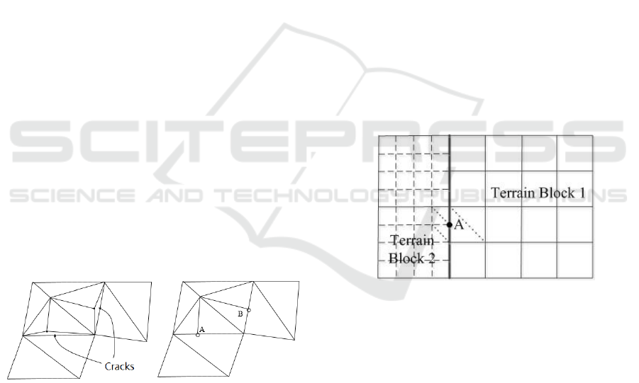
responsible for inducing cracks. Fig. 1(a) is an

example of terrain cracks. In this case, adjustments

will be made to the boundary vertices that belong to

the node that has a higher level of resolution. In Fig.

1(b), the elevations of the A and B vertices (which

belong to the upper left node) have been recalculated

and reevaluated according to the boundary vertices of

the adjacent node.

(a) (b)

Figure 1: Crack elimination via the adjustment of elevation

values: (a)Crack generation and (b) T-joints.

2.2 Inadequacies of the Current

Method

Elevation adjustment-based crack elimination

algorithms can be used to remove cracks by adjusting

the elevation of mesh boundary vertices without

requiring triangulation. However, certain aspects of

these algorithms remain problematic.

(1) Cracks can be generated by adjacent nodes

with LoDs that are different by more than 1, but this

scenario is not accounted for in current elevation

adjustment-based crack removal algorithms.

Furthermore, this scenario is likely to occur in

complex terrain areas during real-time 3D terrain

rendering.

(2) During crack removal, real-time CPU

calculations are required to traverse the entirety of the

terrain. This process is a highly time consuming when

massive terrain data are involved.

(3) After the vertex elevations around the cracks

have been adjusted by these algorithms, certain

discontinuities will become apparent in the lighting of

the terrain. In Fig. 2, for instance, the right side of

boundary vertex A (terrain block 1) is not included in

any triangular mesh. The right side of vertex A will

therefore be excluded during the calculation of vertex

normals, which subsequently leads to discontinuities

between the vertex normal of A and the adjacent

vertices. This issue will subsequently affect the

terrain lighting calculations in 3D scenes and lead to

errors in illumination-based terrain analyses.

Figure 2: Lighting calculation for a pair of terrain blocks.

3 IMPROVED TERRAIN CRACK

REMOVAL METHOD

The crack removal method we have proposed is

suitable for large boundary LoD differences and

consists of three primary steps: (1) the construction of

terrain quadtree structures that contain edge and angle

adjacency information and an algorithm for real-time

updates, (2) the elimination of cracks caused by large

differences in LoD, and (3) the calculation and

updating of the vertex normals of terrain blocks.

A Method of Terrain Crack Removal Suited for Large Differences in Boundary LoD

3.1 The Construction of a Quadtree

Structure That Contains Adjacency

Information and the Dynamic

Updating of This Structure

Differences in the rendering precision of adjacent

terrain nodes are the root cause of terrain cracks (Fu

et al, 2012.WIESEMANN et al, 2005). Therefore, the

key to eliminating terrain cracks is the accurate

recognition and determination of terrain node

adjacencies when real-time LoD terrain rendering is

implemented based on quadtree features. The

following definitions have been provided to facilitate

the description of the algorithm.

(1) Terrain nodes, such as A1 and A2 in Fig. 3, are

simply referred to as tiles. A unified code is used to

describe the LoD, row and column of each tile, i.e.,

Tilecode = (LoD, TileX, TileY). Each tile contains

M×M vertices, with M being a positive integer that

represents the number of grid points on a given edge.

(2) In a terrain quadtree, "parentless" nodes, such

as C1 in Fig. 3, are referred to as root nodes, and

"childless" nodes, such as C2, C6 and C7 in Fig. 3,

are referred to as leaf nodes.

(3) The tiles that surround each tile are

categorized either as edge neighbors or corner

neighbors based on their spatial relationships. Edge

neighbors can be classified as left edge neighbors

(LN), upper edge neighbors (UN), right edge

neighbors (RN), and bottom edge neighbors (DN).

Corner neighbors may be classified as left upper

corner neighbors (LUN), right upper corner neighbors

(RUN), right lower corner neighbors (RDN), and

lower bottom edge neighbors (LDN). An example of

these spatial relationships is illustrated in Fig. 4.

(4) In a quadtree structure, "child" nodes on the

upper left, upper right, bottom right and bottom left

corners of a "parent" node are referred to as LUChild,

RUChild, RDChild and LDChild, respectively.

Figure 3: Terrain quadtree structure.

Figure 4: Definitions of adjacency relationships.

3.2 The Construction and Dynamic

Updating of Quadtree Structures

During the rendering of a 3D terrain scene, terrain

quadtrees will be constructed and dynamically

updated according to the rules of view-dependent

LoD control (Feng et al, 2010. Lindstrom et al, 2001).

A change in view will therefore affect the merging

and splitting of leaf nodes in a quadtree. For instance,

Fig. 5(a) describes a terrain quadtree that corresponds

to the view being close to the upper-left part of the

terrain, and Fig. 5(b) illustrates the changes in the

quadtree when the view shifts from the upper-left part

of the terrain to the bottom-left part. When the

quadtree changes from Fig. 5(a) to Fig. 5(b), the

LDChild1 tile in Fig. 5(b) will split into four

"children" tiles, and the LUChild2, RUChild2,

RDChild2 and LDChild2 tiles in Fig. 5(a) will be

merged. This process corresponds to the rendering of

the "parent" tile (LUChild1).

The dynamic updating of adjacency information

associated with the generation of "children" tiles or

the merging of "parent" tiles (when the "parent" tile

is being rendered) is a crucial step in crack removal.

This adjacency processing algorithm can be divided

into two modules according to the intrinsic

characteristics of each leaf node: an algorithm that

processes the adjacency information of split leaf

nodes, and an algorithm that processes the adjacency

information of merged leaf nodes.

Since terrain cracks only occur at inter-tile

boundaries, the ultimate purpose of crack removal is

to ensure that the four edges and corners of a tile are

consistent with those of adjacent tiles. The

assessment of adjacency information is based on the

spatial and positional relationships of the tiles. To

facilitate the computations of the crack removal

algorithm, we define a marker called "Dirty" for the

adjacency information of each edge and corner of

every tile. Dirty has two possible states: active or

GISTAM 2019 - 5th International Conference on Geographical Information Systems Theory, Applications and Management

sleeping. The specific procedure is given in the

following subsection.

(a)

(b)

Figure 5: An illustration of a terrain quadtree being

updated: (a) View located at the upper-left part of the terrain

and (b) View located at the bottom-left part of the terrain.

3.2.1 The Processing of Adjacency

Information for Split Leaf Nodes

The location of a split leaf node relative to its "parent"

tile is determined, and the adjacency information of

the former is then acquired using its location and

spatial/positional relationships. The determination of

the corner and edge neighbors of a "child" tile located

at the upper-left corner of a "parent" tile (LUChild) is

described below.

(1) The determination of edge neighbors and their

states

Since the split leaf node is an upper left "child"

tile, the tiles that neighbor the split leaf node on its

right and bottom edges must belong to the same

"parent" and have the same level of resolution. Hence,

the "Dirty" crack removal markers of the following

edges are set to the sleeping state: the right and

bottom edges of the current tile, the left edge of the

right-edge neighbor, and the upper edge of the

bottom-edge neighbor. As the left and upper-edge

neighbors have different "parents" than the current

tile, the next step is to find the "parents" of the left

and upper edge neighbors of the current and to

subsequently perform calculations for the left and

upper-edge neighbors of the current tile. The "Dirty"

crack removal markers of the edges associated with

all the previously mentioned tiles are then set to the

active state.

(2) Determination of corner neighbors and their

states

As before (i.e., during the determination of edge

neighbors and their states), the bottom-right corner

neighbor of the upper-left corner "child" tile has the

same parent as the current tile and therefore the same

level of resolution. Thus, the "Dirty" crack removal

markers of the bottom-right corner of the current tile

and the upper-right corner of the bottom-right corner

neighbor are set to the sleeping state. Since the upper

left, upper right, and bottom left corner neighbors

belong to different "parents" than the current tile, the

next step is to search for the parents of the upper-left,

upper-right and bottom-left corner neighbors of the

current tile. The corner neighbors of the current node

are then identified, and the "Dirty" crack removal

markers of the corners associated with the current tile

are set to the active state.

3.2.2 The Processing of Adjacency

Information for Merged Leaf Nodes

Since four "children" are merged to form a "parent",

it is necessary to update the adjacency information of

the neighbors of these "children" in sequential

fashion. Again, the "child" tile in the upper-left corner

(LUChild) is used as an example to explain this

process.

(1) The determination of edge neighbors and their

states

The adjacency information of the right-edge and

bottom-edge neighbors does not require further

processing because these neighbors have the same

parent as the current LUChild tile and because these

three tiles are also simultaneously merged. If the left-

edge (LN) and upper-edge (UN) neighbors have the

same LoD as the LUChild tile, the adjacency

information of the LN and UN tiles will change after

the 4 "children" tiles have been merged. The right-

edge neighbor of LN and the upper-edge neighbor of

UN are set as the parent of LUChild. If LN and UN

have "children" tiles, the adjacency information of

their associated edges will then need to be recursively

updated. The "Dirty" markers of the corresponding

edges are also simultaneously set to the active state.

(2) The determination of corner neighbors and

their states

A Method of Terrain Crack Removal Suited for Large Differences in Boundary LoD

As before, the adjacency information of the

bottom-right corner neighbor is not processed since it

has the same "parent" as the current tile (LUChild). If

the upper-left corner neighbor (LUN) has the same

LoD as LUChild, the bottom-right corner neighbor of

LUN is then designated the "parent" of LUChild. If

LUN has any "children", the adjacency information

of the relevant corners then needs to be recursively

updated. If an upper-right corner neighbor (RUN) or

bottom-left corner neighbor (LDN) exists and has the

same LoD as LUChild, the corner adjacencies related

to these tiles must be set to null since they are not

spatially adjacent to the corners of the "parent" of

LUChild (like the O and UN2 tiles in Fig. 4).

Similarly, if RUN and LDN have children, their

corner adjacencies also need to be recursively

updated.

3.3 The Removal of Cracks with Large

Differences in Lod

To satisfy the requirements for the real-time

rendering of massive terrain data, terrain frustum

culling is used to perform a preliminary investigation

of the range of tiles that require crack removal when

the terrain renders and quadtrees of each frame are

being constructed. The adjacent tiles and “Dirty”

state of the newly added leaf nodes are determined;

the nodes that have an active “Dirty” state may

contain cracks, and these are stored in the crack repair

set (CrackTileVector). After the preliminary

investigation is complete, crack removal without LoD

difference constraints is performed on the tiles of

CrackTileVector.

Our crack removal algorithm without LoD

difference constraints can be summarized as follows.

Since terrain cracks can only occur at tile boundaries,

the (four) edges and corners of some given tile are

sequentially processed, and linear interpolation is

used to ensure that the node elevations of the tile that

is being processed are consistent with the node

elevations of the adjacent tiles (which may have

different LoDs). The steps in processing the left edge

of a tile are used as an example to explain the specific

processes of the proposed algorithm.

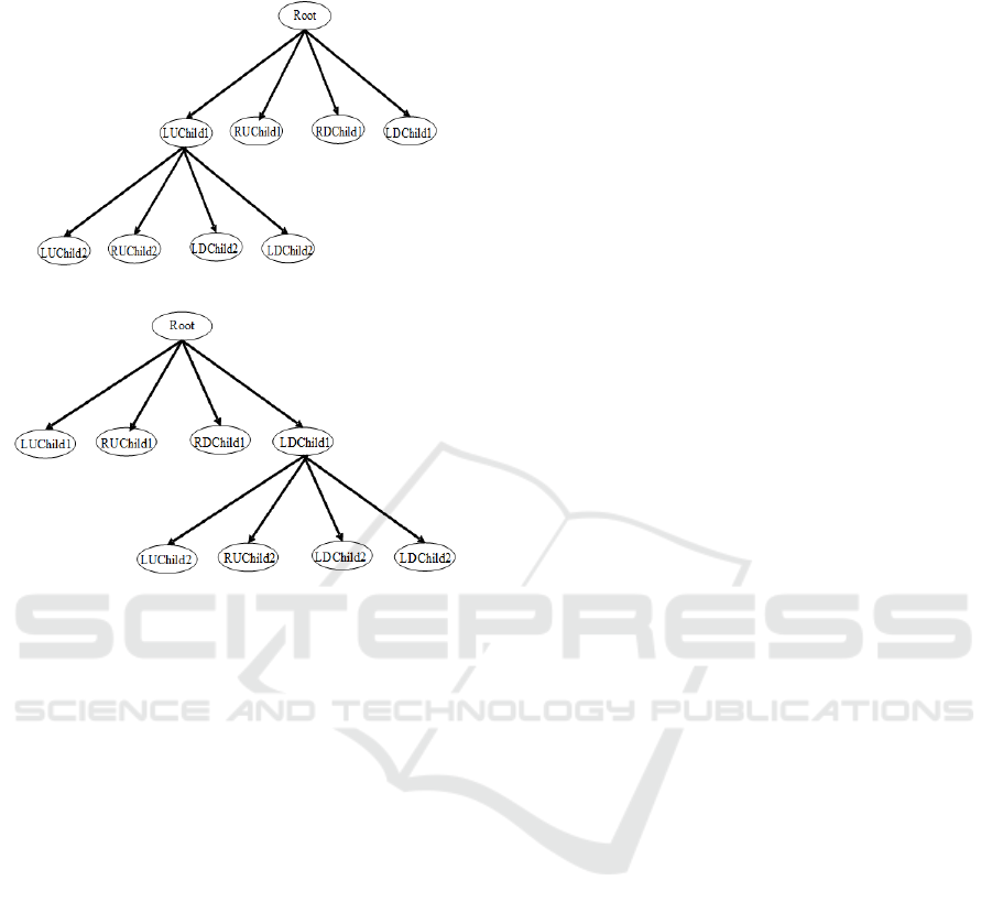
Step 1: Investigate the left-edge neighbor (a leaf

node) of the current tile using dynamically updated

tile adjacency information.

If the current node is N, the adjacency array of the

left neighbor of N is Lvec() (the left-edge neighbor

can exist in various configurations, as shown in Figs.

6(a), 6(b) and 6(c); nevertheless, the processing

procedure is the same in each case). To find the left-

edge neighbor of N in a 3D terrain scene, each

member of the Lvec(array) is checked for “children”.

If a member has “children”, the upper-right and

bottom-right “children” of this member (LChild1

and LChild2, respectively) are assigned to the current

node (N) and treated as the left-edge neighbor of N.

LChild1 and LChild2 are then recursively processed

using these steps until a leaf node is reached and

recorded in the neighbor array, LYvec[]. After the

left-edge neighbor of N has been configured, the

right-edge neighbor of the left-edge neighbor is

simultaneously designated N.

Node of the current tile

The left neighbor node of the currently

displayed scene

(a)

Node of the current tile

The left neighbor node of the

currently displayed scene

(b)

Node of the current tile

The left neighbor node of the currently

displayed scene

(c)

Figure 6: Possible configurations for the left-edge neighbor

of a tile: (a) N and L have the same LoD, (b) N has a greater

LoD than L and (c)N has a lower LoD than L.

Step 2: For the array of left-edge neighbors

(LYvec[]),perform the crack removal operation.

GISTAM 2019 - 5th International Conference on Geographical Information Systems Theory, Applications and Management

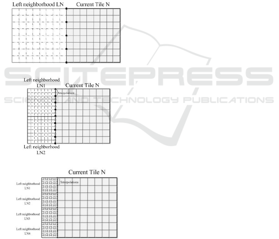
If there is only one node in LYvec[], the left-edge

neighbor and N then have the same LoD, and the

vertex relations between the tiles have a strict one-to-

one correspondence, as shown in Fig. 7(a). In this

case, every vertex on the inter-tile boundary can be

directly traversed to determine whether the vertices

have the same elevation. If the elevations are not

equal, the elevation of N is used as a reference, and

the elevation values of the vertices are assigned to the

corresponding vertices of the corresponding

neighbors. If LYvec[] only has 2 nodes and the LoDs

of N and its neighbor are different by 1, the relation-

ship between the boundary vertices of these tiles is

then described by Fig. 7(b). Additionally, in this case,

the length of two neighboring grids is exactly the

length of a single N grid. Equidistant linear interpola-

(a)

(b)

(c)

Figure 7: Possible configurations for the left-edge neighbor

of a tile: (a)Same LoD, (b)Difference of 1 in LoD and

(c)Difference of 2 in LoD.

ion is then performed on the vertices of N to obtain

the midpoint elevations between each pair of vertices

on the boundary of N; these elevation values are then

assigned to the neighboring vertices. If LYvec has 4

nodes and the difference between the LODs of N and

the neighbor node is n (n > 1), the relationship

between vertices of these tiles is as shown in Fig. 7(c)

(n = 2). This figure illustrates that the length of two

grids in the adjacent tile is 1/n the length of a grid in

N. The grid points of N that are closest to the

neighboring tile are then calculated, and the grid

edges of N are divided in half to form 2n nodes. The

linear interpolation algorithm is used to calculate the

elevations of every node, which are then assigned to

the neighboring vertices.

Since the vertex normals of the boundary mesh

vertices must be recalculated, the “Dirty” markers

of vector normals corresponding to vertices that still

require crack removal are set to the active state.

The proposed crack removal algorithm can be

used without any constraints regarding the difference

in boundary LoD between adjacent nodes. In

addition, our method does not require the rendering

of additional terrain patches, which helps to preserve

actual changes in terrain elevation.

3.4 The Updating of Vertex Normals in

Boundary Areas

Lighting discontinuities may occur at mesh

boundaries after the elevations of vertices at terrain

cracks have been adjusted (Han et al, 2012). After the

terrain cracks have been removed, the vertex normals

of the boundary vertices that participated in the crack

removal operation must be recalculated and re-

evaluated. This process can be described as follows.

Step 1: CrackTileVector is sequentially traversed,

and all the vertices on the four edges of each tile are

processed to determine whether the “Dirty” marker

of the vertex normal is set to the active state. If the “

Dirty ” marker is active, proceed to Step 2;

otherwise, continue to the next vertex.

Step 2: Investigate the 8 vertices that are

connected to this vertex by a triangular mesh, e.g., the

8 vertices around A in Fig. 8. If any of these vertices

are missing, proceed to Step 3 to pad the vertices;

otherwise, proceed directly to Step 4.

Step 3: Vertex padding. Like the crack removal

algorithm, the first step in the padding process is to

determine the LoD difference between the current tile

and an adjacent tile. An analogous subdivision is

performed via linear interpolation of the grids of the

A Method of Terrain Crack Removal Suited for Large Differences in Boundary LoD

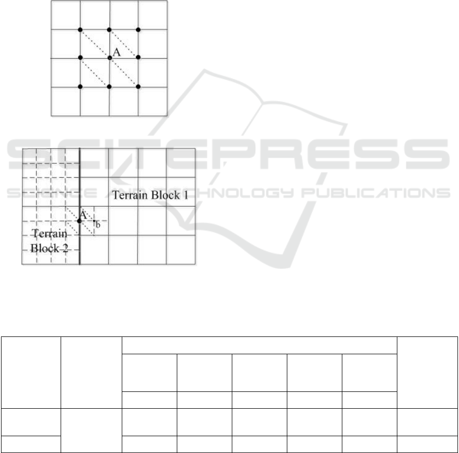
tile with the lower LoD to generate a corresponding

set of vertices in the former tile. Fig. 9 shows that the

grids around the boundary of terrain block 1 should

be subdivided, so that a vertex (b) can be identified

on the right side of boundary point A to participate in

the construction of a triangular mesh.

Step 4: Using the current vertex as the center, the

normal components of each of the 8 directions from

the current vertex are sequentially calculated. These

components are then summed and normalized.

Finally, the vertex normals of the current vertex are

evaluated according to the results of these

calculations.

Figure 8: The vertices associated with point A.

Figure 9: Analogous subdivision of boundary grids.

4 EXPERIMENTS AND

ANALYSIS OF RESULTS

4.1 Experimental Data and

Environment

The proposed terrain crack removal algorithm was

embedded in the NewMap software platform

developed by the Chinese Academy of Surveying and

Mapping. The effectiveness of the method was then

tested using the terrain data from a typical

mountainous region in Sichuan Province. The

elevation data were obtained from the Shuttle Radar

Topography Mission (SRTM), with a coordinate

range of (97.5°～108.5°E, 26.2°～34.1°N); the

horizontal and vertical resolutions of the data were 90

m and 0.1 m, respectively. The image data were

derived from the terrestrial remote sensing data from

Landsat. The multiresolution elevation and image

quadtree pyramids were constructed using NewMap

TerrainPublish software, and the sizes of these

pyramids were 15.76 GB and 63.34 GB, respectively.

The hardware environment of this experiment was a

PC equipped with a 2.60 GHz Pentium Dual Core

E5300 CPU, 1.96 GB of internal storage, and a

Nvidia GeForce 6800 graphics card.

4.2 Results and Analysis

4.2.1 Validating the Reliability of the

Proposed Method

The proposed method was compared to the elevation

adjustment-based crack removal method (i.e., the

conventional method) to validate the reliability of our

method. A random region was selected from the

experimental data to compare the effectiveness of

these methods in removing terrain cracks. The results

of this experiment are shown in Table 1.

Table 1: Comparison of crack removal effectiveness.

Total number

of tiles

Number of terrain cracks

Rate of

terrain crack

removal

LoD

difference

of 1

LoD

difference

of 2

LoD

difference

of 3

LoD

difference

of 4

Total

number of

cracks

2057

1080

384

3585

Conventiona

l method

17072

2057

57.38%

Our method

2057

1080

384

3585

100%

GISTAM 2019 - 5th International Conference on Geographical Information Systems Theory, Applications and Management

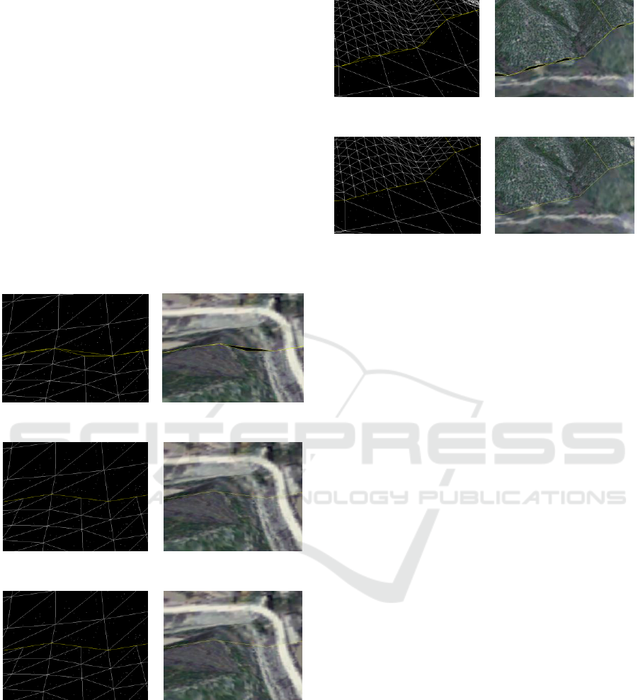
Table 1 shows that there are large differences in

LoD around the boundaries where terrain cracks

occur. Terrain cracks with an LoD difference of 1

account for 57.38% of the total number of terrain

cracks in the experimental area. The conventional

method successfully eliminates all terrain cracks

with an LoD difference of 1 but is unable to process

terrain cracks with LoD differences greater than 1.

Our method is able to completely eliminate all

terrain cracks with LoD differences of 1 and terrain

cracks with LoD differences greater than 1.

Specifically, a terrain crack removal rate of 100%

was achieved in this area using the proposed method.

Figs. 10, 11 and 12 illustrate the effectiveness of the

aforementioned methods in removing terrain cracks

with LoD differences of 1, 2 and greater than 2,

respectively.

(a) (b)

(e) (f)

Figure 10: Comparison of our method and the conventional

method for the removal of terrain cracks with an LoD

difference of 1:(a)Terrain crack with an LoD difference of

1, (b)Visualization of the terrain crack, (c)Results of crack

removal using the conventional method, (d)Results of crack

removal using the conventional method, (e)Results of crack

removal using our method and (f)Visualized result of crack

removal using our method.

(a) (b)

Figure 11: The effectiveness of our method in removing

terrain cracks with an LoD difference of 2 : (a)Terrain

cracks with an LoD difference of 2, (b)Visualization of

terrain cracks, (c)Results of terrain crack removal using our

method and (d)Visualized result of terrain crack removal

using our method.

Figs. 10 and 11 clearly show that both the

aforementioned methods can effectively eliminate

terrain cracks that have an LoD difference of 1, and

the proposed method is also suitable for removing

terrain cracks that have LoD differences of 2, the

complex terrain in the studied region is accurately

reproduced by the processed terrain structures.

4.2.2 Validation of Lighting Continuity

By changing the rules applied for tile splitting, the

tiles that are rendered in a scene will have the same

LoD, which ensures that cracks cannot occur

throughout the entirety of the terrain scene. In this

case, the lighting of the meshes around tile boundaries

is continuous, and this is referred to as the theoretical

reference value. However, under normal tile splitting

rules, the tiles that are rendered in a scene can have

different LoDs, and these are the actual values of the

vertex normals (lighting) after the crack removal

process has been implemented. A comparison was

made between the vertex normals calculated by our

method and the conventional method for the tile

boundaries of a terrain block to inspect the continuity

of the lighting values in each case. The theoretical

values and actual (post-crack removal) values of the

vertex normals are shown in Table 2.

A Method of Terrain Crack Removal Suited for Large Differences in Boundary LoD

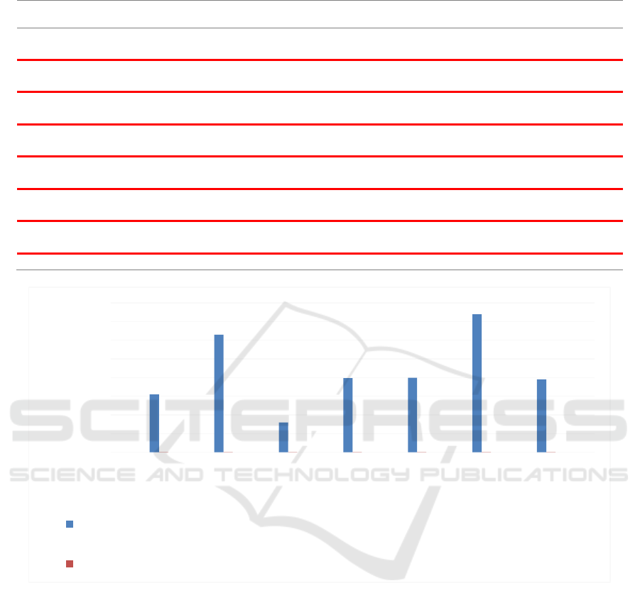
Table 2: Comparison of vertex normal at tile boundaries.

Vertex

number

Theoretical value (X, Y, Z)

Vertex normals of the

conventional method (X, Y, Z)

Vertex normals of our method

(X, Y, Z)

(0.630410,0.279561,0.724174)

(0.623360,0.294948,0.724174)

(0.724351,0.134632,0.676158)

(0.623450,0.294758,0.724174)

(0.615934,0.310157,0.724174)

(0.608136,0.325179,0.724174)

(0.649363,0.623852,0.434898)

(0.608129,0.325194,0.724174)

(0.599973,0.340006,0.724174)

(0.591448,0.354628,0.724174)

(0.639341,0.398756,0.657447)

(0.591449,0.354630,0.724172)

(0.582567,0.369035,0.724174)

(0.563758,0.397176,0.724174)

(0.737288,0.423349,0.526481)

(0.563761,0.397176,0.724172)

(0.573335,0.383221,0.724174)

(0.543590,0.424360,0.724174)

(0.415249,0.628213,0.657964)

(0.543588,0.424363,0.724174)

(0.553841,0.410892,0.724174)

(0.533012,0.437573,0.724174)

(0.743681,0.577819,0.336250)

(0.533012,0.437573,0.724174)

(0.522113,0.450522,0.724174)

(0.499378,0.475598,0.724174)

(0.657243,0.261486,0.706864)

(0.499381,0.475595,0.724174)

(0.510899,0.463199,0.724174)

Figure 12: Comparison between the boundary vertex normals calculated by our method and the conventional method.

The red underlines in Table 2 serve to highlight

differences between the theoretical and actual values

of the vertex normals. The X, Y and Z components of

the vertex normals that were calculated by the

conventional method and our method were subtracted

from the reference values, and the absolute values of

these results were then summed to produce the bar

chart shown in Fig. 12. This figure shows that the

vertex normals calculated by our method for all 15

vertices (which are tile boundary vertices) are

essentially identical to the theoretical values. Notably,

only minor differences were observed at the 5th

decimal place and beyond, which are negligible in the

calculation of terrain tile lighting. However, there are

significant differences between the vertex normals

calculated by the conventional method and the

theoretical values, particularly for vertices 2, 4, 6, 8,

10, 12 and 14. These differences will lead to

discontinuities in the lighting of tile boundaries.

4.2.3 Efficiency Validation

The efficiency of our method was validated by setting

the view to roam around the experimental area for 20

minutes. During this time, the total number of tiles,

number of cracks and time consumed by crack

removal in every frame of the terrain rendering

process was randomly sampled at 12 instants. The

results are shown in Table 3.

0.1

0.2

0.3

0.4

0.5

0.6

0.7

0.8

1 2 3 4 5 6 7 8 9 10 11 12 13 14 15

Sum of absolute vertex normal

differences

Vertex number

Sum of absolute differences between the reference values and those of the conventional

method

Sum of absolute differences between the reference values and those of our method

GISTAM 2019 - 5th International Conference on Geographical Information Systems Theory, Applications and Management

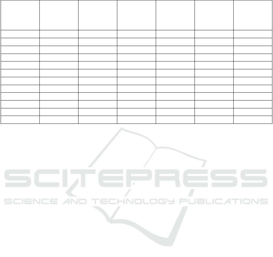
Table 3: Crack removal statistics.

Time point (s)

Frames rendered

Total number of

tiles

Total number of

cracked tiles

Proportion of

cracked tiles

Time

consumption of

our method (ms)

Time

consumption of

the conventional

method (ms)

8.13

1025

244

12.30%

0.670

7.425

24.70

3458

273

2.93%

0.104

8.105

50.35

6643

396

4.04%

0.672

9.362

64.13

8721

355

5.92%

1.302

7.853

86.03

12474

473

2.75%

0.314

9.537

113.73

16149

440

4.32%

0.531

9.046

258.79

36231

492

5.28%

2.623

9.951

275.1

41264

212

10.38%

1.451

6.433

419.21

54498

516

4.65%

1.534

9.427

507.17

66439

460

6.09%

2.352

8.854

790.74

104378

543

9.02%

2.858

9.364

898.84

119546

316

9.81%

1.692

7.223

Table 3 shows that the proposed method requires

less computational time than the conventional method

because our method only computes the “parent”

nodes obtained from newly split or merged leaf nodes

during terrain crack removal; hence, only the tiles that

correspond to terrain cracks are processed. During

crack removal with the conventional elevation

adjustment-based method, the entirety of the terrain

quadtree must be traversed; therefore, all the tiles

must be processed when this method is used. This

approach consumes more computational time, and the

average processing time of the conventional method

is approximately 8 times that of our method.

5 CONCLUSIONS AND

DISCUSSION

In this work, we have proposed a terrain crack

removal method that is able to handle large

differences in boundary LoD. This method fully

exploits the features of quadtree structures and the

implicit adjacency relationships of parent and child

nodes. Additionally, terrain crack removal and the

updating of boundary vertex normals occur in real

time. With this method, the elimination of terrain

cracks will no longer be limited by differences in

boundary LoD. The following conclusions were

drawn from the validations and comparative analyses

that were performed using terrain data from a typical

mountainous region in Sichuan Province.

(1) Our method is applicable at boundaries where

the difference in LoD is equal to 1 and complex

terrain areas where the LoD difference between

adjacent tiles is greater than 1.

(2) The continuity of terrain lighting is ensured by

our method through the recalculation and re-

evaluation of boundary vertex normals after the crack

removal process, thereby overcoming the lighting

discontinuities that hinder the use of the conventional

crack removal method.

(3) The efficiency of our method is, on average,

eight times greater than that of the conventional

method because the proposed method does not

traverse the entirety of the terrain quadtree during

crack removal, which saves a substantial quantity of

computational time.

The method that is proposed in this work is

suitable for terrain rendering based on quadtree

structures. However, further research must be

performed to investigate the suitability of the method

for other terrain mesh models, such as triangular

meshes and binary tree models.

ACKNOWLEDGEMENTS

This research was funded by a project supported by

the National Key Research and Development

Program of China (Grant No. 2016YFF0201305) and

National Natural Science Foundation of China (Grant

No. 41871375).

A Method of Terrain Crack Removal Suited for Large Differences in Boundary LoD

REFERENCES

Bulatov D, Häufel G, Meidow J, et al. 2014. Context-based

automatic reconstruction and texturing of 3D urban

terrain for quick-response tasks. Isprs Journal of

Photogrammetry & Remote Sensing, 93(7):157-170.

Feng W W, Kim B U, Yu Y, et al. 2010. Feature-preserving

triangular geometry images for level-of-detail

representation of static and skinned meshes. Acm

Transactions on Graphics, 29(2):11-22.

Fu W, Ge Z H, Li W H. 2012. A terrain rendering method

with dynamic error metric for flight simulation. Journal

of Jilin University (Science Edition), 50(6): 1175-1178.

Han L T, Kong Q L, Dai H L, et al. 2012. Optimization of

normal calculation of regular grid terrain based on

OpenGL. Science of Surveying and Mapping, 37(5):17-

19.

Han M, Tang S T, Li Y. 2008. Real-time visualization

algorithm of large-scale terrain. Computer Engineering,

34(13):270-272.

Ke X L, Zeng J. 2005. Dynamic rendering for LOD virtual

terrain using quadtree. Bulletin of Surveying and

Mapping, (6):10-13.

Li Q, Dai S L, Zhao Y J, et al. 2013. A block LOD real-time

rendering algorithm for large scale terrain. Journal of

Computer-Aided Design & Computer Graphics,

25(5):000708-713.

Liu Y, Guan A D, Li J. 2010. A model for massive 3D

terrain simplification based on data block partition and

quad-tree. Acta Geodaetica et Cartographica Sinica,

39(4):410-415.

Nie J L, Liu S, Guo D L, et al. 2013. GPU-accelerated fast

rendering method for multi-resolution geometry image.

Journal of Computer-Aided Design & Computer

Graphics, 25(1):101-109.

P Lindstrom, V Pascucci. 2001. Visualization of Large

Terrains Made Easy. Proceedings of IEEE

Visualization. 363-370.

Wan M, Liang X, Zhang F M. 2015. Improved crack

removing algorithm for quad-tree terrain rendering.

Journal of System Simulation, 27(7):1520-1525.

Wang D C, Wan W G, Tang J Z, et al. 2007. Preprocessing

LOD algorithm for large scale terrain based on

restricted quadtrees. Computer Engineering and

Applications, 43(24):107-109.

WIESEMANN T, SCHIEFE LE J, KUBBAT W. 2005.

Multi-resolution Terrain Depiction on an Embedded

2D/3D Synthetic Vision System. Aerospace Science

and Technology, 9 (6):517-524.

Xu M Z. 2005. Research on Real-Time Rendering for Large

Scale Terrain. Geomatics and Information Science of

Wuhan University, 30(5):392-395.

Yang Y, Wang C, Gao Y, et al. 2014. Large Scale Terrain

Real-Time Rendering on GPU Using Double Layers

Tile Quad Tree and Cuboids Bounding Error Metric.

Open Automation & Control Systems Journal, 2014,

6(1):1378-1388.

Yin Y, Chen G J, Wu W. 2006. An algorithm of avoiding

crack for rendering parting terrain. Journal of

Computer-Aided Design & Computer Graphics,

18(10):1557-1562.

Zhao X S, Fan D Q, Wang J J, et al. 2012. Seamless

expression of the global multi-resolution DEMs based

on degenerate quadtree grids. Acta Geodaetica et

Cartographica Sinica, 41(6):918-925.

Zhao Y B, Shi J Y. 2002. A fast algorithm for large scale

terrain walkthrough. Computer-Aided Design &

Computer Graphics, 14(7):624-628.

Zheng X, Liu W, Lu C L, et al. 2013. Real-time dynamic

storing and rendering of massive terrain with GPU.

Journal of Computer-Aided Design & Computer

Graphics, 25(8):1146-1152.

GISTAM 2019 - 5th International Conference on Geographical Information Systems Theory, Applications and Management