
Time Zone Impact for Traffic Flow Analysis of Ahmedabad City in
India
Tsutomu Tsuboi
Global Business Development Office, Nagoya Electric Works Co., Ltd, 29-1 Metoku Shinoda, Ama, Japan
Keywords: Traffic Flow, Traffic Density, Traffic Volume, Traffic Congestion, Traffic Occupancy.
Abstract: This paper describes time zone impact for traffic flow analysis in an one of major city in India based on one
month real traffic monitoring big data. The target city is Ahmedabad of Gujarat state where is located in the
west part of India. The current population in Ahmedabad is about 7.8 Million and it is one of rapid economic
growing city. These days, the traffic congestion in the city become one of major issues. In order to analyse
traffic congestion, large amount of the traffic big data is needed and it is collected through the traffic
monitoring camera. The measurement of the data is traffic density, traffic occupancy and average of speed of
vehicles which is measured at the road by every minute. The traffic data in emerging countries is not well
analyzed so far because of difficulty of collecting traffic data. Author has a chance to involve one of traffic
project which provides traffic condition to the drivers through traffic information boards and makes
suggestions for avoiding traffic congestion. The current judgement of the traffic congestion is based on the
occupancy of the road which is one of traffic flow parameters. This occupancy is not so accuracy sometimes
because of difficulty of 100 % vehicle sensing. In this paper, it describes the time zone basis traffic flow
analysis in the traffic flow characteristics such as traffic density to average vehicle speed curve, traffic density
to traffic volume curve, and traffic volume to average vehicle speed. This analysis is able to identify the effect
of time zone to traffic flow condition and provide more appropriate occupancy level for traffic congestion.
1 INTRODUCTION
1.1 Background
The aim of this research is about how to analyse real
traffic condition in a developing county, which is still
not quite so much before because of lack of
infrastructure for collecting data.
Author has a chance to involve one of traffic
management project at Ahmedabad city of Gujarat
state in India since 2014. The project is installing
traffic monitoring cameras at several major roads in
the city and showing real time traffic condition
through the electrical traffic information sign boards
along the roads. The electrical traffic information sign
board is usually called “Variable Message Signs
(VMS)”, which becomes popular especially on
express highway. The traffic condition is calculated
from collecting traffic data through traffic monitoring
cameras and showing the traffic condition by three
classes’ level, heavy congestion, slightly congested,
and smooth condition by coloured lines red, yellow,
and green. The drivers are able to understand the
traffic condition of the road and also recognize other
alternative detour to their destination. This project has
been started from October 2104 with 14 traffic
monitoring cameras and 4 VMSs. And now we have
31 cameras and 11 VMSs as total these days.
On the basis of collecting traffic data, we convert
into the basic traffic flow characteristics—traffic
density (K) – average vehicle speed (V) or K-V curve,
traffic density (K) – traffic volume (Q) or K-Q curve,
and traffic volume (Q) – average vehicle speed (V) or
Q-V curve. After achieving these characteristics
analysis, we have the following two features.
The first one is that each curve has different value
based on traffic condition of each road, but the shape
of curves are similar. There is a clear boundary
observation line in each curve which looks like traffic
flow curve from traffic flow theory. But the plotted
position of measurement data are widely spread under
the boundary observation line, which is different from
other advanced countries. The followings sections
explain this uniqueness of traffic flow characteristics
in Ahmedabad.
388
Tsuboi, T.
Time Zone Impact for Traffic Flow Analysis of Ahmedabad City in India.
DOI: 10.5220/0007708103880395
In Proceedings of the 5th International Conference on Vehicle Technology and Intelligent Transport Systems (VEHITS 2019), pages 388-395
ISBN: 978-989-758-374-2
Copyright
c
2019 by SCITEPRESS – Science and Technology Publications, Lda. All rights reserved
The second one is to show the traffic condition
transition by time zone basis traffic flow analysis.
This feature provides idea about traffic congestion
mechanism from the basic traffic flow characteristics.
The last part, it propose the appropriate occupancy
level for the traffic congestion.
1.2 Related Studies
In terms of the study of traffic flow analysis in the
emerging countries, there are several related studies
these days such as in India. Goutham.M has proving
data analysis at National Highway in Hyderabad. It
shows trend of traffic condition and comparison with
Indian Road standard IRC-106-1990 but
measurement points are only two Highways and
volume is two days with five CCTVs. In Salim.A et
al study, it describes traffic congestion condition by
headway measurement in Chennai. But measurement
point is only one city road and four days data with one
hour for each. It is also limited measurement data.
There are more advanced technology available by
using information communication technology (ICT).
For example, there is so called Probing technology by
collecting traffic data with Global Positioning System
(GPS) in side vehicles. This study is estimation by
using probing vehicle behavior but this case study is
limited number of probe data and a study in the
advanced country i.e. Italy. For probing technology
based traffic analysis, there are many case studies in
the vehicular ad hoc network (VANET) environment.
These research are useful to estimation traffic safety
application especially in the congested traffic
condition. In VANET environment, the advanced
communication technology is sued such as Dedicated
Short Radio Communication (DSRC), Cellular phone
network like Long term Evolution (LTE), 3G, 4G,
and 5G etc. Most of the advanced network
communication technology has just been released in
the advanced countries and will be installed in new
manufacturing vehicles in future.
2 TRAFFIC MONITORING
SYSTEM AND MEASUREMENT
2.1 Traffic Monitoring System
The total system configuration of Ahmedabad traffic
management consists of 14 traffic monitoring
cameras and 4 VMSs at the first stage in October in
2014. The traffic data is collected by the traffic
cameras and is send to the clod server. The traffic
condition is calculated based on the collected data
and then the results of calculation analysis of the
traffic condition is transpired to VMSs. The total
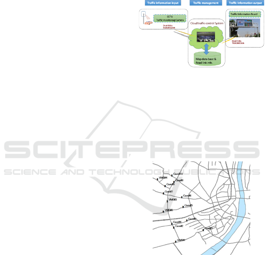
system configuration is illustrated in Figure.1.
Figure 1: Traffic Management System Configuration.
The location of the traffic management system is
the west side of Ahmedabad city where there are new
business buildings and new shopping centre and more
crowded by people. Therefore .it becomes heavy
traffic jams in the morning and the evening every day.
The installation place of each cameras and VMSs is
shown in Figure.2. In Figure.2, Cam# means Camera
and its number. And VMS# means VMS and its
number. The number of cameras is 10 in Figure.2 but
it is also setting with VMS system. So the total
number of camera is 14 (10 plus 4).
Figure 2: Traffic Management System Location.
2.2 Measurement Data
In this section, let’s show several examples of traffic
characteristics based on measurement traffic data.
The Figure.3 (A) shows the traffic density (K) to
average vehicle speed (V) or K-V curve at the
Camera#1 in June 2015. And the Figure.3 (B) shows
K-Q curve at the Camera#1 and Fig.3 (C) shows Q-V
curve at Camera#1. Those three curves are called the
Time Zone Impact for Traffic Flow Analysis of Ahmedabad City in India
389
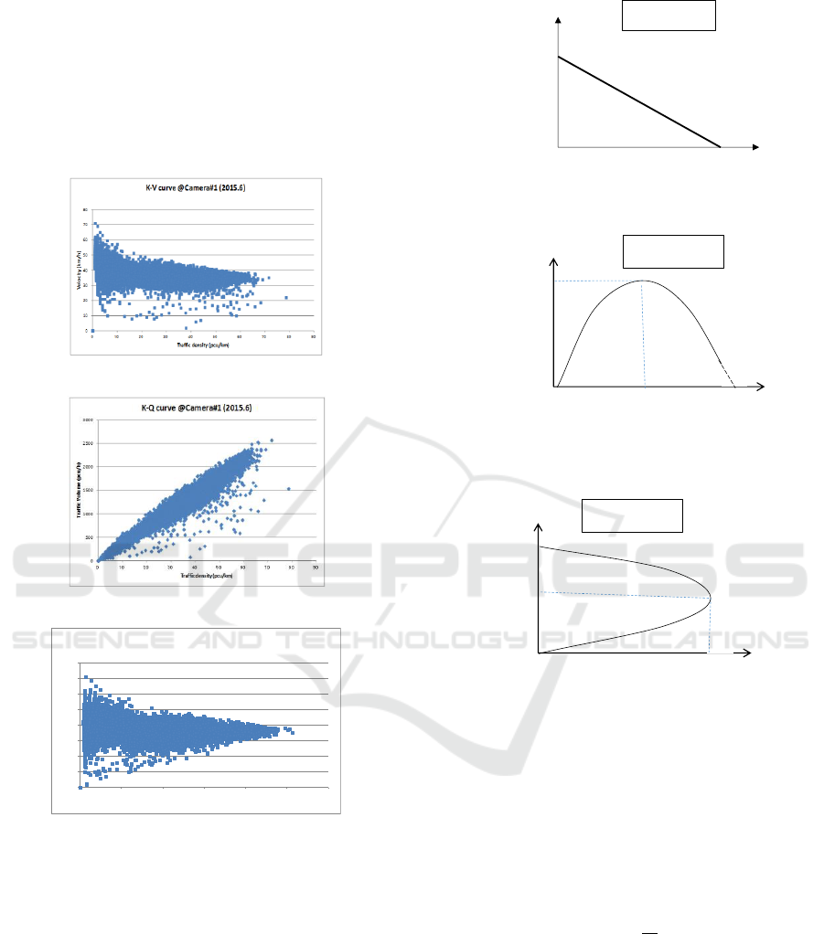
fundamental diagram about the traffic flow
characteristics.
In terms of K-V curve, there are several theoretical
curves which explains traffic condition. The typical
curve is known as Greenshields curve. This curve is
linier relationship between the traffic density (K) and
average vehicle speed (V). The illustration of
Greenshields curve is shown in Figure.4 (A).
(A) K-V curve at Camera#1.
(B) K-Q curve at Camera#1.
(C) Q-V curve at Camera#1.
Figure 3: Basic Traffic Flow curves at Camera#1.
When it is compare between Figure.3 (A) and
Figure.4 (A), the boundary observation line in
Figure.3 (A) is similar with the Greenshields curve in
Figure.4. However there are wide spread
measurement data under its boundary observation
line in Figure.3 (A). This is also same condition in K-
Q curve and Q-V curve compared with Figure.3 (B)
and Figure.4 (B), and Figure.3 (C) and Figure.4 (C).
It is also same results from other measurement points.
We will see this reason in detail at the chapter 3.
(A) Theoretical K-V curve.
(B) Theoretical K-Q curve.
(C) Theoretical Q-V curve.
Figure 4: Theoretical Traffic Flow curves.
2.3 Theoretical Traffic Flow Equations
From Figure.4 (A), the average vehicle speed (v) is
calculated by the equation (1) of the traffic density (k)
under Greenshields curve.
(1)
where v
f
is free flow speed and k
j
is the jam
density at speed equal to zero condition. The equation
(2) is given from the traffic theory.
(2)
0
10
20
30
40
50
60
70
80
0 500 1000 1500 2000 2500 3000
Velocity (
km/h)
Traffic Volume (pcu/hr)
Q-V curve @Camera#1 (2015.6)
vf
kj
0
K-V curve
k
v
Traffic density
velocity
kj
0
k
q
qc
kc
K-Q curve
Traffic density
Traffic volume
vj
0
v
q
qc
vc
Q-V curve
Traffic volume
Velocity
VEHITS 2019 - 5th International Conference on Vehicle Technology and Intelligent Transport Systems
390
After eliminating v between equation (1) and (2),
the equation (3) is achieved.
(3)
Then equation (4) is taken by transforming
equation (3).
(4)
Based on the result of equation (4), theoretical K–
Q curve and is shown in Figure.4 (B). It is quadratic
curve of traffic density (k). As same manner as
reaching equation (4), equation (5) is taken by
eliminating traffic density (k) between equation (1)
and (2).
(5)
It is quadratic curve of traffic speed (v) and it is
shown in Figure.4 (C) but x axis and y axis are
opposite position.
From comparison between Figure.3 (A), (B) (C)
and Figure.4 (A), (B) (C), the boundary observation
line in each Fig.4 curve follows each equation (1), (4),
and (5). The uniqueness from actual measurement
data plot in Figure.3 is widely spread under each
boundary observation line. This is big different with
the experience in the advanced countries’ data.
3 MESUREMENT DATA
ANALYSIS
3.1 Actual Traffic Condition
In this chapter, it describes the analysis with actual
traffic condition during 24 hours for one month in
June 2015. The Figure.5 (A) shows time zone base
traffic volume (q) transition at Camera#1 from 7:00
am to 6:00 am in the next day and Figure.5 (B) shows
time zone base average vehicle speed from 7:00 am
to 6:00 am in the next day. The measurement data is
plotted by average, weekday average, Saturday
average, and Sunday average.
(A) Time Zone based Traffic Volume at Camera#1.
(B) Time Zone based Vehicle speed at Camera#1.
Figure 5: Actual Traffic Condition at Camera#1.
In case of Camera#2, Figure.6 (A) and (B) show
time zone based traffic volume and speed.
(A) Time Zone based traffic volume at Camera#2.
(B) Time Zone based Vehicle speed at Camera#2.
Figure 6: Actual Traffic Condition at Camera#2.
From both Figure.5 and Figure.6, there are two
peak of traffic volume in the morning and in the
evening. But the vehicle speed drop in the evening at
0
500
1000
1500
2000
7 8 9 10 1112 1314 15 16 1718 19 20 2122 23 0 1 2 3 4 5 6
Traffic Volume
(pcu/hr)
Time Zone
Traffic Volume @ Camera#1 (2015.6)
Qave Qweek Qsa Qsu
0
10
20
30
40
50
7 8 9 1011 12 13 14 15 16 17 18 19 20 21 22 23 0 1 2 3 4 5 6
Velocity
(km/hr)
Time Zone
Velocity @ Camera#1 (2015.6)
Vave Vweek Vsa Vsu
0
200
400
600
800
1000
1200
1400
7 8 9 10 11 12 13 14 15 16 17 18 19 20 21 22 23 0 1 2 3 4 5 6
Traffic Volume
(pcu/hr)
Time Zone
Traffic Volume @ Camera#2 (2015.6)
Qave Qweek Qsa Qsu
0
5
10
15
20
25
30
35
7 8 9 10 11 12 13 14 1516171819 20 21 22 23 0 1 2 3 4 5 6
Velocity
(km/hr)
Time Zone
Velocity @ Camera#2 (2015.6)
Vave Vweek Vsa Vsu
Time Zone Impact for Traffic Flow Analysis of Ahmedabad City in India
391
Camera# 2 is significant compared by that of
Camera#1, which means there is heavy traffic jam in
the evening at Camera#2.
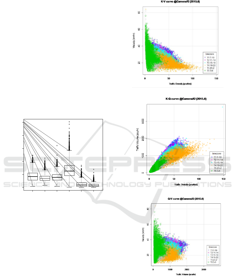
3.2 Time Zone based Fundamental
Diagram
In this section, there is more detail traffic congestion
condition observation by considering the relationship
between congestion condition and its traffic
fundamental diagram of the time zone. In order to
simplify characteristics, it defines six time zones from
T1 to T6 as shown in Table 1 rather than each hourly
data like Figure.5 and 6.
Table 1: Time Zone Classification.
Zone Name
Time Zone
T1
7:00 – 10:00
T2
11:00 - 14:00
T3
15:00 - 18:00
T4
19:00 - 22:00
T5
23:00 - 2:00
T6
3:00 - 6:00
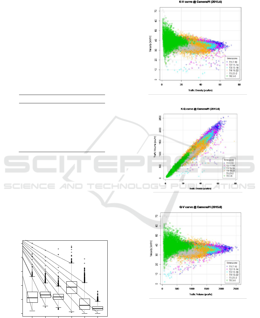
As the first case study, it describes the
fundamental characteristics of Camera#1. In terms of
the traffic congestion condition, it is used the
occupancy percentage by time zone in Japan. The
Figure.7 shows the occupancy value at Camera#1 by
time zone basis. According to Figure.7, the most
congested condition is occurred at Time Zone T4,
when it starts from 19:00 to 22:00. The traffic volume
at T4 is the second peak of traffic volume but the
average vehicle speed is slightly lower than that of
Time Zone T2 of which traffic volume is first peak at
Figure 7: Occupancy at Camera#1.
Camera#1. Therefore it can be said that the traffic
condition at T4 is more congested at Camera#1.
(A) K-V curve at Camera#1.
(B) K-Q curve at Camera#1.
(C) Q-V curve at Camera#1.
Figure 8: The Time Zone basis Fundamental Diagram at
Camera#1.
In case of the fundamental diagram at Camera#1
by Time Zone, there are K-V curve, K-Q curve, and
T1:7-10 T2:11-14 T3:15-18 T4:19-22 T5:23-2 T6:3-6
0
10
20
30
40
50
Occupancy @ Camera#1 (2015.6)
Time Zone
Occupancy (%)
VEHITS 2019 - 5th International Conference on Vehicle Technology and Intelligent Transport Systems
392
Q-V curve at Camera#1 in Figure.8. It is clear that the
area under the boundary curve is the data from
congested time zone T1, T2, and T4 from Figure.8
(A). There are also lots of measurement data under
the boundary observation line in each Time Zone.
From Figure.8 (B) and (C), the critical traffic volume
happens at Time Zone T1, which is the first traffic
volume peak of the day. This condition is clear from
Figure.5 and 6. But in case of the fundamental traffic
characteristics, it is clearer by using divided six time
zone. The grey colour area is mixed measurement
plots. In Figure.8, each dot is real measurement data
by every minute during all days in June 2015. So total
number of plots is 43,200 points (=60 minutes x24
hours x30 days).
In case of Camera#2 where we see more traffic
congestion condition, the occupancy percentage is
shown in Figure.9.
Figure 9: Occupancy at Camera#2.
And the fundamental diagram of Camera#2 is
shown in Figure.10. The trend of each fundamental
curves of Camera#1 and Camera#2 is similar. But
there is particular differentiation, especially in case of
K-V curve. According to Figure 6 (B), the vehicle
speed during 18:00 to 22:00 (T4) goes down, which
means that traffic condition becomes congested.
Therefore in Time Zone basis Fundamental Diagram,
T4 (Brown colour) portion is lower position in each
curves.
(A) K-V curve at Camera#2.
(B) K-Q curve at Camera#2.
(C) Q-V curve at Camera#2.
Figure 10: Time Zone basis Fundamental Diagram at
Camera#2.
T1:7-10 T2:11-14 T3:15-18 T4:19-22 T5:23-2 T6:3-6
0
20
40
60
80
100
Occupancy @ Camera#2 (2015.6)
Time Zone
Occupancy (%)
Time Zone Impact for Traffic Flow Analysis of Ahmedabad City in India
393

4 CONCLUSIONS
From the view point of big volume measurement data,
this is the first time to make a detail traffic flow
analysis in one of major mega city in India. The
Ahmedabad city of Gujarat state is a one of typical
rapid economical grow area in India. Author analyses
one moth traffic flow data based on the traffic flow
theory. By using the uniqueness of the traffic flow
characteristics, it is valid to consider the boundary
observation line in the fundamental diagram from its
traffic flow theory equation. The following are
conclusion of this study.
The boundary observation line of the
fundamental diagram is representative of its
traffic flow characteristics.
The area under the boundary observation line of
the fundamental diagram comes from data of
congested traffic condition time zone.
The critical traffic volume comes from the peak
traffic volume time zone.
The traffic flow model is different from those of
the advanced countries by measurement data
spread plot.
This study is the begging of the analysis of traffic
flow in developing country and it provides different
thoughts about traffic congestion reason. And it is
necessary to have more study about this kind of
research such as driving behaviour, road line effect,
different city case study, long term data collection.
ACKNOWLEDGEMENTS
This study also underwent the ID16667556 of the
International Science and Technology Cooperation
Program (SATREPS) challenges for global
challenges in 2016.
Special appreciation to Mr.Kikuchi.C and
Mr.Mallesh.B of Zero-Sum ITS India for providing
traffic data in Ahmedabad.
REFERENCES
Goutham.M, Chanda.B, 2014. Introduction to the selection
of corridor and requirement, implementation of IHVS
(Intelligent Vehicle Highway System) In Hyderabad,
International Journal of Modern Engineering Research,
Vol.4, Iss.7, pp.49-54.
Salim.A, Vanajakshi.L, Subramanian.C, 2010. Estimation
of Average Space Headway under Heterogeneous
Traffic Conditions, International of Recent Trends in
Engineering and Technology, Vol. 3, No. 5
Carli.R, Dotoli.M, Epicoco.N, 2017. Monitoring traffic
congestion in urban areas through probe vehicle: A
case study analysis, Wiley Online Library, 2017.
https://onlinelibrary.wiley.com/doi/pdf/10.1002/itl2.5.
Ahmed.S.H, et al, 2016. Controlled data and Interest
Evaluation in Viheicular Named data Networks, IEEE
Trans Vehicle Technology, 65(6), pp.395-3963.
Tsuboi.T, Oguri.K, 2016, Traffic Flow Analysis in
Emerging Country, Information Processing Society of
Japan Journal, Vol.57, No.4, pp.1284-1289.
Ohashi.K, Yanagisaa.Y, Takagishi.S, etal. 2009. Traffic
System Engineering, Corona Publising Co. Ltd., p.94.
Greenshields B. D. 1935. A Study of Traffic Capacity, Proc.
H. R. B., 14, pp.448-477.
Kubota.H, Ohashi.T, Takahashi,.K, 2010. Traffic
Engineering and Traffic Planning, Riko Publishing
Co., Ltd., pp.24-25.
Tsuboi.T, Oguri.K, 2016, Analysis of Traffic Flow and
Traffic Congestion in Emerging Country, Information
Processing Society of Japan Journal, Vol.57, No.12,
pp.2819-2826.
Sadakata.M, 975. Measurement of Congestion Degree in
Rood Traffic, The Society of Instrument and Control
Engineers, No.1, Vo.11.
APPENDIX
There is little reference about the Boundary
Observation method in the Appendix. The Figure.A-
1 shows k-v curve at driving lane of Camera#1 with
approximate line by Boundary Observation method
and Least Square method. The Least Square method
is generally used in Statics Analysis for understand
the trend of measurement data. From Figure.A-1, the
equation by Least Square method is right rising curve,
which does not follow the traffic flow theory. On the
other hand, the equation by Boundary Observation
method is right downward curve and follows the
traffic flow theory. In this example, the Boundary
Observation method shows the traffic flow limitation
of each road.
In case of K-Q curve at Camera #1, the traffic flow
characteristics is shown in Figure.A-2. The Boundary
Observation equation of K-Q curve is q= - 0.3516(k –
80)2+2250. Therefore the jam density kj=160. From
equation (4), the free speed v
f
=56.25. When the
Least Square equation of K-Q curve from Figure.A-
2, the traffic volume q= -0.022k
2
+ 31.213k + 4.689 =
-0.022(k-709.4)
2
+503233.2. The jam density k
j
=1418.772. Then free speed v
f
= 31.21. It does not
match with v
f
of Figure.A-1.
As the result, it is able to say that the Least Square
method shows the trend of traffic measurement data
VEHITS 2019 - 5th International Conference on Vehicle Technology and Intelligent Transport Systems
394
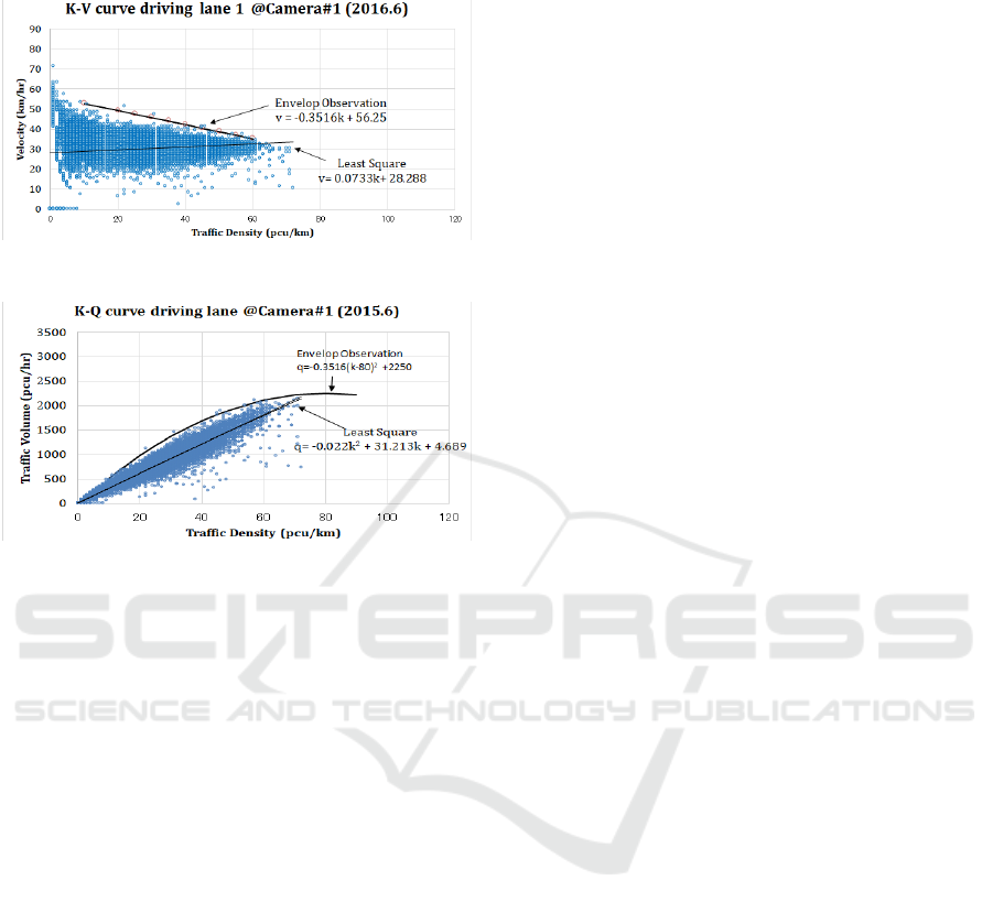
but it does not provide the traffic parameter data such
as jam density and free speed.
Figure A-1: K-V curve driving lane at Camera#1.
Figure A-2: K-Q curve driving lane at Camera#1.
Time Zone Impact for Traffic Flow Analysis of Ahmedabad City in India
395
