MultiMagNet: A Non-deterministic Approach based on the Formation of

Ensembles for Defending Against Adversarial Images

Gabriel R. Machado

, Ronaldo R. Goldschmidt

and Eug

enio Silva

Section of Computer Engineering (SE/8), Military Institute of Engineering (IME), Rio de Janeiro, Brazil

Computing Center (UComp), State University of West Zone (UEZO), Rio de Janeiro, Brazil

Keywords: Artiﬁcial Intelligence and Decision Support Systems, Advanced Applications of Neural Networks.

Abstract:

Deep Neural Networks have been increasingly used in decision support systems, mainly because they are

the state-of-the-art algorithms for solving challenging tasks, such as image recognition and classiﬁcation.

However, recent studies have shown these learning models are vulnerable to adversarial attacks, i.e. attacks

conducted with images maliciously modiﬁed by an algorithm to induce misclassiﬁcation. Several works have

proposed methods for defending against adversarial images, however these defenses have shown to be inefﬁ-

cient, since they have facilitated the understanding of their internal operation by attackers. Thus, this paper

proposes a defense called MultiMagNet, which randomly incorporates at runtime multiple defense compo-

nents, in an attempt to introduce an expanded form of non-deterministic behavior so as to hinder evasions by

adversarial attacks. Experiments performed on MNIST and CIFAR-10 datasets prove that MultiMagNet can

protect classiﬁcation models from adversarial images generated by the main existing attacks algorithms.

1 INTRODUCTION

The advances that Deep Neural Networks have pre-

sented in recent years has been impulsed mainly by

the increasingly necessity to analyse and interpret a

massive and diversiﬁed amount of data (Obermeyer

and Emanuel, 2016). Currently, information systems

which make use of intelligent resources to support de-

cisions in safety-critical environments involving com-

puting vision tasks, such as (i) biometric recognition

for users authentication (Derawi et al., 2010) (Bae

et al., 2018), (ii) identiﬁcation of handwritten dig-

its or characters (Srivastava et al., 2019) (Tolosana

et al., 2018) and (iii) surveillance systems (Ding et al.,

2018), are among the various applications of Deep

Neural Networks.

Nevertheless, recent work have demonstrated that

the performance of Deep Neural Networks, which

can even overcome the human perception (Karpathy,

2014), has signiﬁcant drop in face of adversarial im-

ages (Szegedy et al., 2013) (Goodfellow et al., 2015)

(Papernot et al., 2016a) (Carlini and Wagner, 2017c).

Adversarial images contain malicious perturbations

generated by an attack algorithm, usually minimal

and imperceptible to human eyes, but can lead learn-

ing algorithms to misclassiﬁcation. This attack is

known as adversarial attack (Madry et al., 2017). The

facility that attackers have into fooling classiﬁers can

result in wide-range losses and accidents in real world

scenarios, menacing the use of these learning mod-

els on several security-critical applications (Klarreich,

2016).

In order to minimize the harmful effects of the

adversarial attacks, several defenses have been pro-

posed. Many defense approaches consist of detect-

ing the existence of possible perturbations in im-

ages before they misclassify learning models (Xu

et al., 2018) (Gong et al., 2017) (Metzen et al., 2017)

(Hendrycks and Gimpel, 2017). However, works

such as (Carlini and Wagner, 2017a) and (He et al.,

2017) have demonstrated that these defenses have

limitations in terms of (i) their ability to detect ad-

versarial images generated by diferent attacks algo-

rithms and/or (ii) their utilization of deterministic

approaches, i.e. defenses that, at each execution,

always uses the same procedure, which facilitates

the attacker’s understading of the defense’s modus

operandi.

As a means of reducing the dependence of the de-

fense for speciﬁc attack algorithms and hindering the

prediction of its behaviour by the attacker, a recent

work has developed a defense, called MagNet (Meng

and Chen, 2017). MagNet is a non-deterministic de-

fense which randomly chooses at runtime a compo-

Machado, G., Goldschmidt, R. and Silva, E.

MultiMagNet: A Non-deterministic Approach based on the Formation of Ensembles for Defending Against Adversarial Images.

DOI: 10.5220/0007714203070318

In Proceedings of the 21st International Conference on Enterprise Information Systems (ICEIS 2019), pages 307-318

ISBN: 978-989-758-372-8

307

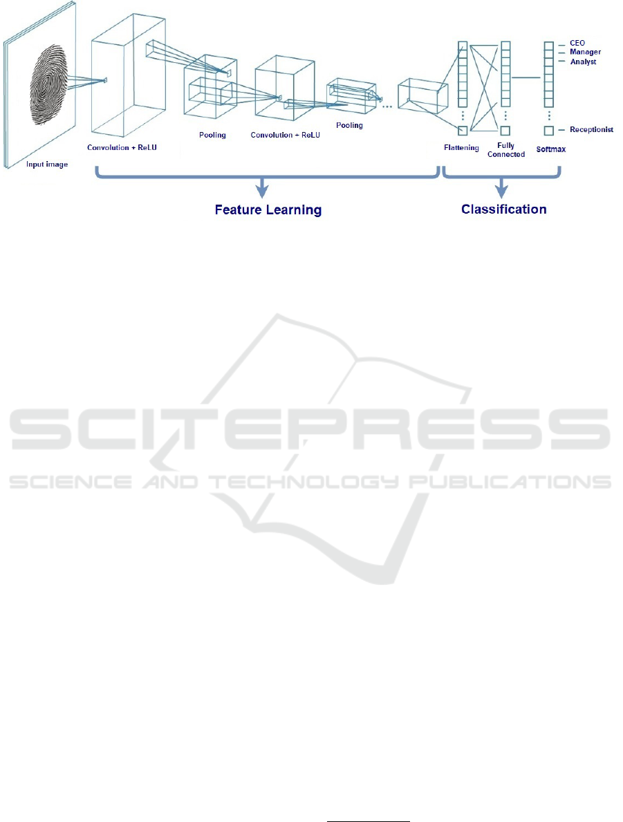
Figure 1: An example of a CNN containing several convolutional layers.

nent, used to compute a threshold needed to classify

the input images as legitimate or adversarial. After-

wards, the images classiﬁed as legitimate are recon-

structed by another component before being sent to

the classiﬁer. Despite presenting some promising re-

sults before various adversarial attacks, (Carlini and

Wagner, 2017b) have shown that, even with the non-

deterministic effect provided by the random selection

of a defense component, MagNet can be evaded by

adversarial images. Thus, this work raises the hypoth-

esis that the selection of multiple defense components

can amplify the non-deterministic effect, reducing the

predictability of the defense method’s behaviour, be-

coming it more robust than MagNet against different

adversarial attacks algorithms.

Therefore, this paper proposes MultiMagNet, an

adversarial image detection method which arranges

ensembles at runtime by randomly choosing multiple

defense components, implemented as autoencoders.

Experiments performed on MNIST (LeCun et al.,

1998) and CIFAR-10 datasets (Krizhevsky and Hin-

ton, 2009) indicate the veracity of the hypothesis by

showing that MultiMagNet has presented better re-

sults than MagNet in the majority of attack scenarios

evaluated.

This paper is structured as follows: Section 2

brings the needed background to understand the work.

Section 3 summarizes the main defense methods

against adversarial images available in literature. Sec-

tion 4 details the proposed defense method. Section

5 describes the experiments performed and discusses

the obtained results. Finally, Section 6 brings the ﬁnal

considerations, highlights the main contributions of

this work and indicates suggestions for future works.

2 BACKGROUND

2.1 Convolutional Neural Networks

The Convolutional Neural Networks (CNNs), a spe-

cial type of Deep Neural Network, are the state-of-

the-art learning models in image classiﬁcation and

recognition tasks (He et al., 2016) (Hu et al., 2017)

and, for this reason, they have become the prime tar-

get of adversarial attacks. The CNNs, unlike the con-

ventional neural networks, are able to learn automat-

ically the main features of a image by reducing its

representation space. After the extraction of the most

important features, the fully-connected layer acts in a

way similar to a regular neural network, with the dif-

ference of producing as an output the probabilities of

the input image belonging to each class of the prob-

lem being studied. These probabilities are computed

using the softmax function at the last layer of the neu-

ral network. Figure 1 shows an example of a CNN

architecture. More details about the CNNs can be ob-

tained at (Goodfellow et al., 2016).

2.2 Autoencoders

Autoencoders are neural networks trained to recon-

struct an input x, generating as an output an approx-

imation x

, with the smallest reconstruction error as

possible (Goodfellow et al., 2016). Formally, an au-

toencoder ae = d ◦ e comprises two components: (i)

an encoder e : S → H and a decoder d : H →

S, where

S is the input space, H is the compressed space learnt

by the encoder component and

S represents the input

Adapted from https://www.mathworks.com/discovery/

convolutional-neural-network.html. Accessed in June 23,

2018.

ICEIS 2019 - 21st International Conference on Enterprise Information Systems

308

space reconstructed by the autoencoder. The recon-

struction error ER

ae(x)

is the difference between the

input x and its reconstructed version x

= ae(x) as de-

ﬁned by Equation 1, where p is the distance metric:

ae(x)

= ||x − ae(x)||

(1)

Autoencoders usually are used for (i) dimension-

ality reduction and (ii) feature learning, once they pre-

serve only the most important features of the data

(Goodfellow et al., 2016).

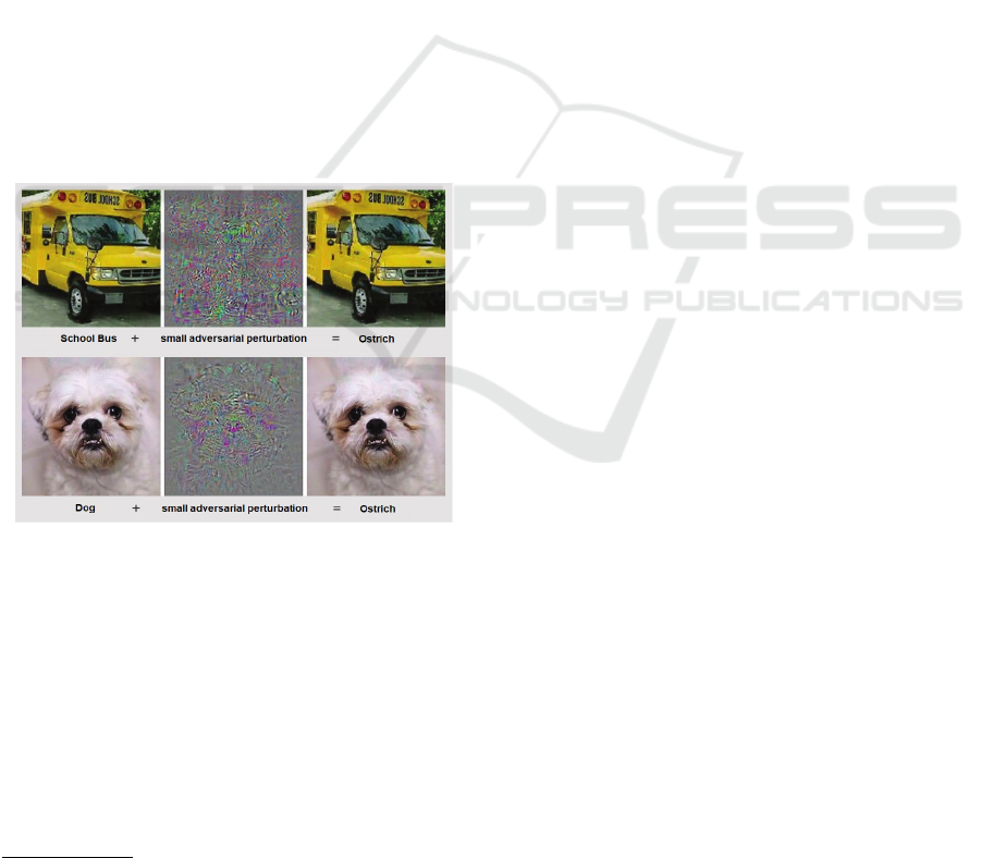
2.3 Adversarial Images

An adversarial image is a image which contains a

minimal perturbation

, oftentimes imperceptible to

human eyes, generated by a malicious algorithm in

order to induce learning models to misclassiﬁcation

(see Figure 2). Formally, given a model F trained

using legitimate images, x an input image such that

x ∈ R

w×h×c

, where w and h are the dimensions of im-

age x and c its quantity of color channels, it is gen-

erated an image x

adv

, such that x

adv

= x + δx, where

δx is the perturbation and, in a succeeded adversarial

attack, F(x) 6= F(x

Figure 2: Malicious and usually imperceptible perturba-

tions in a input image can induce trained models to mis-

classiﬁcation. Adapted from (Klarreich, 2016).

2.4 Adversarial Attacks

Adversarial attacks are malicious optimization algo-

rithms which generate and insert perturbations into

legitimate images in order to lead previously trained

models to misclassiﬁcation. There are several algo-

rithms available in literature, however, for the exper-

iments performed in this work, it has been used the

A perturbation is a systematic distortion maliciously

generated in an image by an attack algorithm.

four most used adversarial attacks: (i) FGSM, (ii)

BIM, (iii) DeepFool e (iv) CW. These adversarial at-

tacks are explained in the following.

Fast Gradient Sign Method (FGSM) (Goodfel-

low et al., 2015): FGSM is a non-iterative attack al-

gorithm, whose main characteristic is its linear com-

plexity. The linear complexity of FGSM is compu-

tationally efﬁcient, however it contributes to generate

larger perturbations than the ones generated by itera-

tive algorithms. Given an image x ∈ R

w×h×c

, FGSM

generates an adversarial image x

adv

using Equation 2.

adv

= x − ε · sign(∇

J(Θ,x,y)) (2)

In Equation 2, Θ represents the network parame-

ters, y the respective class of x, ε the maximum per-

turbation which can be inserted into the image x and

J(Θ,x,y) is the cost function used to train the net-

work.

Basic Iterative Method (BIM) (Kurakin et al.,

2016a): BIM is the iterative version of FGSM. Unlike

FGSM that executes only a step of size ε towards the

gradient descent, BIM executes several smaller steps

α, where the result is upper bounded by ε in order to

prevent the amount of perturbation does not exceed

the quantity desired by the attacker. Formally, BIM

is a recursive method that computes x

adv

according to

Equation 3:

adv

(

adv

= 0

adv

= x

adv

i−1

− clip(α · sign∇

J(Θ,x

adv

i−1

,y))

(3)

DeepFool (Moosavi-Dezfooli et al., 2016): The

ideia behind DeepFool consists of ﬁnding the closest

decision boundary from a legitimate image x in the

image space. Afterwards, x is subtly perturbated so

as to make it cross the decision boundary and fool the

classiﬁer. Due to the high dimensionality of the im-

age, DeepFool adopts an iterative approach of linear

approximation. In each iteration, DeepFool linearizes

the model around the intermediate x

adv

and computes

an optimal update direction in the linearized model.

Then, x

adv

is updated on this direction by a small step

α.

Carlini & Wagner Attack (CW) (Carlini and

Wagner, 2017c): The CW attack is the state-of-the-art

algorithm to generate adversarial images. Formally,

CW is an iterative attack where, given a CNN F with

Z as the penultimate layer, called logits, and an legit-

imate image x belonging to the class t, CW uses the

gradient descent to solve Equation 4:

minimize ||x − x

adv

+ c · `(x

adv

) (4)

where the cost function `(x

adv

) is deﬁned in Equation

MultiMagNet: A Non-deterministic Approach based on the Formation of Ensembles for Defending Against Adversarial Images

309

`(x

adv

) = max(max{Z(x

adv

)

: i 6= t} −Z(x

adv

)

,−con f )

(5)

In Equation 5, the hyperparameter con f indicates

the conﬁdence level of the CW attack. Higher val-

ues of con f usually produce adversarial images with

greater ability to fool classiﬁers, however, these im-

ages will also contain more perturbations within.

2.5 Jensen-Shannon Divergence

The Jensen-Shannon Divergence (JSD) computes the

divergence between two probabilistic distributions P

and Q. In this work, the distributions P and Q are

obtained by the output of softmax layer F of a CNN

where, given two images x and y, P = F(x) and

Q = F(y). P(i) e Q(i) indicate respectively the prob-

abilities of the images x and y belong to the class i.

The value of the JSD metric, given two images x and

y, is computed by Equation 6.

JSD(P ||Q) =

(P||M) +

(Q||M) (6)

where

M =

(P + Q), D

(P||Q) =

∑

P(i)log

P(i)

Q(i)

3 RELATED WORK

The defense of classiﬁcation models against adversar-

ial attacks is not a trivial task and several strategies

have already been proposed in literature. The most

relevent work in this subject and their respective ap-

proaches to defend against adversarial attacks are next

discussed.

Adversarial Training (Szegedy et al., 2013),

(Goodfellow et al., 2015), (Kurakin et al., 2016b),

(Madry et al., 2017), (Kannan et al., 2018): The ad-

versarial training, also known as robust optimization,

is a proactive defense approach

based on data aug-

mentation

to train classiﬁers in a dataset containing

legitimate and adversarial images, thus forcing the

classiﬁcation model to produce correct outputs to the

malicious images. This strategy has two important

limitations: (i) it is computationally expansive and (ii)

Defenses against adversarial images are divided into (i)

proactive defenses, which aim to make models more ro-

bust in classifying adversarial images and (ii) reactive de-

fenses, which act as detectors of adversarial images, pre-

venting them from reaching the classiﬁer.

Procedure performed in a dataset in order to increase

the amount of samples used to train classiﬁcation models.

it is deterministic, once it creates dependencies be-

tween the detection method and the attack algorithms

used in the adversarial training process.

Defensive Distillation (Papernot et al., 2016b): is

a proactive and deterministic defense which trains a

model F in a dataset X containing legitimate samples

and labels Y , generating as output the probabilities

set F(X ). Afterwards, the original labels set Y are

then replaced by the F(X) probabilistic set, and a new

model F

with the same architecture of F is created

and trained with dataset X yet using the probabilis-

tic labels F(X). After training, the obtained model

, called distilled model, produces the probabilis-

tic distilled outputs F

. Classiﬁers using defensive

distillation are based on gradient masking: an effect

that hides the classiﬁer’s gradient in order to hinder

the generation of adversarial images by the attacker

(Papernot et al., 2017). Defenses based on gradient

masking can be easily bypassed since the attacker can

create his own classiﬁer, generate adversarial images

using this classiﬁer and a more elaborated attack al-

gorithm, and ﬁnally transfer these recently generated

images to the distilled classiﬁer (Carlini and Wagner,

2017c).

Feature Squeezing (Xu et al., 2018): reactive de-

fense which is based on the hypothesis that the high

dimensional image spaces facilitates attackers into

generating stronger perturbations. Therefore, the au-

thors basically have used two methods for reducing

the dimensionality of the images, in order to remove

possible perturbations that may be present in them:

(i) color bit depth reduction and (ii) spatial smooth-

ing. Using a classiﬁer and a predeﬁned threshold,

a comparison is performed among the prediction of

the original image x with the predictions of its ver-

sions x

, reduced by the method (i), and x

, reduced

by the method (ii), respectivelly. If one of these

comparisons is above the threshold, x is labeled as

adversarial and disposed before reaching the classi-

ﬁer. Despite presenting good results before CW at-

tack, (He et al., 2017) has shown it is possible to

evade it, mainly because its deterministic architecture,

which always chooses the same dimensionality reduc-

tion techniques at each execution.

MagNet (Meng and Chen, 2017): MagNet is a

reactive and non-deterministic method that is formed

by two defense layers: (i) the detection layer which

rejects, using a predeﬁned threshold, the images far

from the decision boundary, once they contain more

perturbations, and (ii) a reformer layer that receives

the images coming from the detection layer and re-

constructs them in order to remove any undetected

perturbations. After the reconstruction, the image is

sent to the classiﬁer. MagNet chooses randomly two

ICEIS 2019 - 21st International Conference on Enterprise Information Systems

310

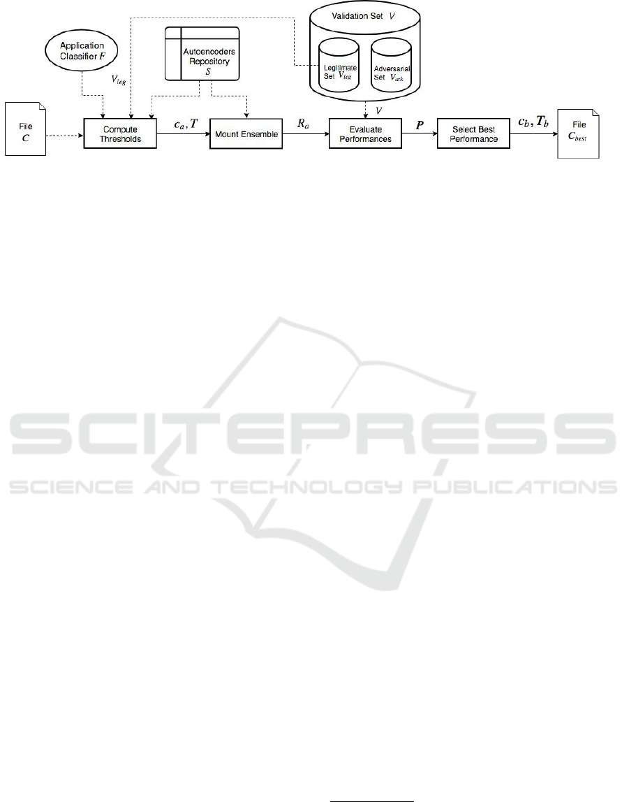
Figure 3: Schematic ﬂowchart of the Calibration Stage.

autoencoders from a repository: one for the detection

layer and the other one for the reformer layer. De-

spite the use of randomness for choosing both autoen-

coders, (Carlini and Wagner, 2017b) has shown that

MagNet can be evaded by adversarial images.

4 PROPOSED DEFENSE

The defense method proposed in this paper, called

MultiMagNet, is an extension of MagNet. The Multi-

MagNet’s operation basically comprises two stages:

(i) the Calibration Stage and (ii) the Deployment

Stage. All the processes which compose the Calibra-

tion Stage are going to be explained ﬁrst. Later, the

processes related to the Deployment Stage will also be

discussed.

4.1 The Calibration Stage

In the Calibration Stage (see Figure 3), all the Multi-

MagNet’s desired combinations of hyperparameters,

predeﬁned by the user as inputs in a ﬁle C, are once

evaluated using the validation set V and the applica-

tion classiﬁer F. At the end of the Calibration Stage,

the best combination of hyperparameters c

∈ C and

the thresholds set T

(computed using the hyperpa-

rameters c

) are then saved in a ﬁle called C

best

. The

ﬁle C

best

, once deﬁned, will prompty provide the best

tuple of hyperparameters c

and the thresholds T

for the Deployment Stage, avoiding unnecessary and

repetitive computation. All the processes related to

the Calibration Stage will be next described in details.

4.1.1 Compute Thresholds

The ﬁrst process, Compute Thresholds, receives as in-

put a ﬁle C, deﬁned beforehand by the user, which

contains his desired set of values to be evaluated for

the following MultiMagNet’s hyperparameters: (i)

the false positive rate set T

f p

, such that t

f p

∈ T

f p

and 0 < t

f p

< 1, (ii) the temperature set K, where

∈ K,k

≥ 1, (iii) the metric set M, which me

∈ M

can be the Reconstruction Error (RE), deﬁned by

Equation 1, or the Jensen-Shannon Divergence (JSD),

deﬁned by Equation 6 (formally, me

∈ {RE,JSD}),

and (iv) the threshold approach set T , where T =

{minTA,MTA}, δ

∈ T . These hyperparameters are

going to be explained in Section 4.1.3. Besides the

ﬁle C, this process also receives as inputs the vali-

dation subset V

leg

containing only legitimate images,

the respository S containing m autoencoders

and the

application classiﬁer F. This process gives as output

the set T , which contains m × c computed thresholds,

where m is the number of autoencoders in repository

S and c is the number of possible combinations of

user-predeﬁned values in the ﬁle C to be evaluated for

the hyperparameter sets T

f p

, K, M and T , such that

c = |T

f p

| × |K| × |M| ×|T | and a ≤ c.

To compute all the m × c thresholds of T , the le-

gitimate images from the validation set V

leg

were ini-

tially reconstructed for each autoencoder s

∈ S, i ≤ m,

forming the V

set, where V

= {vl

|vl

= s

),v

∈

leg

}, and s

) represents the image v

reconstructed

by the autoencoder s

. Next, the classiﬁcation thresh-

olds are deﬁned by RE or JSD metrics, according to

the current hyperparameter δ

Regarding the metric RE, it has been used Equa-

tion 1 to compute the reconstruction errors of each

legitimate image v

and its reconstructed version vl

(where, in Equation 1, x = v

, ae(x) = vl

and p = 1),

thus forming the RE

array. After computing all the

reconstruction errors in V

leg

set using the autoencoder

, the values in RE

array are then sorted in de-

scending order and the hyperparameter t

f p

∈ T

f p

applied

, giving as result the threshold τ

= RE

[t],

where t is the corresponding index, such that t =

f p

× |V

leg

On the other hand, for the metric JSD, it has been

All of the m autoencoders in S are previously trained

in the training dataset Tr, which contains only legitimate

images.

The false positive rate t

f p

represents the percentage of

legitimate images which can be misclassiﬁed as adversarial.

MultiMagNet: A Non-deterministic Approach based on the Formation of Ensembles for Defending Against Adversarial Images

311

necessary to obtain the probabilistic softmax outputs

from the last layer of the application classiﬁer (rep-

resented by a CNN) for each legitimate image from

leg

and its respective reconstruted version. It is worth

mentioning that the softmax outputs are related to the

classes of the original classiﬁcation problem. The

Equation 7 describes the softmax function used.

F(l

) =

exp(l

)

∑

j=1

exp(l

)

(7)

In Equation 7, F represents the softmax layer of

the application classiﬁer, l, also known as logits, rep-

resents the output from the penultimate layer of the

application classiﬁer, i represents the corresponding

index of the class with respect to the original clas-

siﬁcation problem and n means the total number of

classes relating to the original classiﬁcation problem.

The hyperparameter k

∈ K (where k

≥ 1) is used

to normalize the values of l

e l

, in order to prevent

saturation (Meng and Chen, 2017). After computing

the softmax outputs corresponding to the legitimate

images from V

leg

subset and their reconstructed ver-

sions V

, it is calculated the Jensen-Shannon Diver-

gence (JSD) from Equation 6, where P = F(v

), Q =

F(vl

). According to (Meng and Chen, 2017), the uti-

lization of the JSD metric is based on the hypoth-

esis that the divergence of the softmax outputs be-

tween an legitimate image x

leg

and its reconstruct

version xr

leg

is usually smaller than the divergence

between the softmax outputs of an adversarial im-

age x

adv

and its reconstructed version xr

adv

, such that

JSD(F(x

leg

),F(xr

leg

)) < JSD(F(x

adv

),F(xr

adv

)). In

a way similar to the RE metric, all the divergences

computed using the legitimate validation set V

leg

and

an autoencoder s

are kept in an array JSD

, which

is also sorted in descending order and t

f p

∈ T

f p

applied, giving as result the threshold τ

= JSD

[t],

where t = t

f p

× |V

leg

Thus, by using the hyperparameters k

∈ K, me

∈

{RE,JSD} and t

f p

∈ T

f p

, all predeﬁned by the user

in ﬁle C, it is produced as output the T set containing

m × c thresholds.

4.1.2 Mount Ensemble

The Mount Ensemble process receives as inputs the

repository S containing m different autoencoders, the

T set containing m×c thresholds and the current com-

bination c

to be tested in V set, where c

∈ C and

= (t

f p

,me

,δ

), a ≤ c. It gives as output an

ensemble R

, which is formed as described as fol-

lows: n autoencoders are randomly chosen from S,

where n < m and n mod 2 = 1 (to ensure no ties in

the vote count). After choosing the n autoencoders,

their respective thresholds are also loaded from T set,

according to the current combination c

, thus forming

the R

set. Formally, R

= {r

,··· ,r

}, where

is the pairwise (r

,τ

), such that r

∈ S, i ≤ n and

∈ T , a ≤ c.

4.1.3 Evaluate Performance

The Evaluate Performance process receives two in-

puts: (i) the ensemble R

and (ii) the validation set

V = V

leg

∪ V

atk

. V

atk

is formed by 2,000 adversar-

ial images generated from the 2,000 legitimate im-

ages in V

leg

set using an attack algorithm atk, where

atk ∈ {FGSM,BIM,DeepFool,CW }.

Each one of the 4,000 images in V is therefore

reconstructed by all the autoencoders in R

set, form-

ing the set V R

. Afterwards, it is used Equation 1

or 6, according to the current metric me

, to com-

pute the metric value set M

. If me

= RE, it is ap-

plied the Equation 1, where x = v

, ae(x) = vr

and

p = 1, such that v

∈ V , vr

∈ V R

. If me

= JSD,

it is applied the Equation 6, where P = F(v

) and

Q = F(vr

),v

∈ V,vr

∈ V R

Finally, each metric value m

∈ M

is compared

to the threshold τ

, which is computed based on the

current value approach of δ

, which can be: (i) min-

imum threshold (minTA) or (ii) multiple threshold

(MTA). When the minTA approach is selected, it is

considered the smallest threshold among all the as-

sociated thresholds for the n autoencoders in R

, i.e.

= min{τ

,τ

,··· ,τ

}. On the other hand, when

is selected the MTA approach, it is considered each

associated threshold for all the autoencoders in R

i.e. τ

∈ {τ

,τ

,··· ,τ

}. When m

≤ τ

, a vari-

able q

leg

(which represents the votes of v

being legit-

imate) counts a vote, otherwise q

adv

counts a vote. By

majority vote, the image is classiﬁed as legitimate if

leg

> q

atk

, otherwise is classiﬁed as adversarial. At

the end of the vote count for each image v

, it is pro-

duced a confusion matrix Ma as deﬁned in Equation

Ma =



T N FN

FP T P



(8)

In Equation 8, the elements TN,FN, FP and T P

in matrix Ma deﬁne respectively the amount of (i)

adversarial images voted as adversarial, (ii) adversar-

ial images voted as legitimate, (iii) legitimate images

voted as adversarial and (iv) legitimate images voted

as legitimate. After computing the c confusion ma-

trices, it is ﬁnally produced as output by the Evaluate

Performance process the P set, formed by c tuples,

where each tuple contains the following three met-

rics: (i) accuracy (ACC), (ii) positive predictive value

ICEIS 2019 - 21st International Conference on Enterprise Information Systems

312

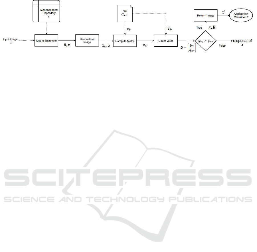
Figure 4: Schematic ﬂowchart of the Deployment Stage.

(PPV) and (iii) negative predictive value (NPV). All

these metrics are formally deﬁned in Equation 9.

ACC =

T N+TP

/T N+FN+FP+T P

PPV =

T N

/T N+FN

NPV =

T P

/T P+F P

(9)

4.1.4 Select Best Performance

The Select Best Performance process receives as in-

put the P set containing c performance tuples. It

is produced as output the ﬁle C

best

which contains

(i) the combination of hyperparameters c

that leads

to the MultiMagNet’s highest accuracy, where c

f p

,me

,δ

) and (ii) the T

set. The T

set, such

that T

⊂ T , contains the n thresholds computed by

using the c

combination of hyperparameters, such

that c

∈ C. The highest accuracy metric on V set has

been chosen to elect the best set of hyperparameters

, since it can describe a more general performance

scenario.

4.2 Deployment Stage

Once calibrated, MultiMagNet is ready to receive in-

put images in the Deployment Stage. After forming

an ensemble R and loading its best set of hyperpa-

rameters c

and the respective thresholds T

from ﬁle

best

, MultiMagNet’s ensemble R can return a verdict

whether an input image x is legitimate or not. The

classiﬁcation made by MultiMagNet is performed by

majority vote, where all the n votes, representing each

autoencoder in R, are counted. In case of being clas-

siﬁed as legitimate, the image x is reconstructed by

an autoencoder randomly selected from R, in order to

remove any undetected perturbations, and afterwards

x is ﬁnally sent to the application classiﬁer F. If x

is classiﬁed as adversarial, MultiMagNet simply dis-

cards it before reaching F. Figure 4 illustrates the ﬁve

processes belonging to the Deployment Stage, and

each of them will be explained in the following.

4.2.1 Mount Ensemble

This process receives two inputs: (i) the repository S

containing m autoencoders and (ii) the input image x

to be evaluated by MultiMagNet. It gives as output

the ensemble R containing n autoencoders chosen at

random, where n ≤ m, n mod 2 = 1.

4.2.2 Reconstruct Image

The Reconstruct Image process receives two inputs:

(i) the input image x and (ii) the ensemble R. It gives

as outputs the image x itself and the X

set, which is

formed by the reconstructed versions xr

of the image

x made by each autoencoder r

∈ R.

4.2.3 Compute Metric

The Compute Metric process receives three inputs: (i)

the input image x, (ii) the X

set containing the n re-

constructed versions of x, such that xr

∈ X

, and the

ﬁle C

best

, which contains the tuple c

of hyperparam-

eters that has led to the best accuracy in Calibration

Stage. In a way similar to the procedures explained

in Sections 4.1.1 and 4.1.3 for computing the metric

values, this process returns the X

set, which contains

the metric values among x and its reconstructed ver-

sions in X

set, which can be computed from Equa-

tion 6 if me

= JSD, where P = F(x) e Q = F(xr

), or

from Equation 1, where ae(x) = xr

and p = 1.

4.2.4 Count Votes

The Count Votes process also works in a very similar

way when compared to the vote count performed by

Evaluate Performance process in Calibration Stage

(see Section 4.1.3). It receives as inputs the X

set

and the T

set provided by C

best

ﬁle. T

contains

the n thresholds that have been deﬁned in Calibra-

tion Stage. It returns q

leg

and q

adv

, which respectively

represent the count of votes for x being legitimate or

adversarial. If q

leg

< q

adv

, the input image x is dis-

carted, otherwise x is sent to the last process, Reform

Image.

MultiMagNet: A Non-deterministic Approach based on the Formation of Ensembles for Defending Against Adversarial Images

313

Table 1: Hyperparameters deﬁned for each attack algorithm.

Attack Datasets and Parameters

FGSM

MNIST: ε = 0.2

CIFAR-10: ε = 0.025

BIM

MNIST: ε = 0.15; α = 0.07; 50 iterations

CIFAR-10: ε = 0.025; α = 0.01; 1,000 iterations

DeepFool

MNIST: overshoot = 0.02; max iter = 50

CIFAR-10: overshoot = 0.02; max iter = 50

MNIST: con f = 0.0; binary searches = 1; lrate = 0.2; initial const = 10, max iter = 100

CIFAR-10: con f = 0.0; binary searches = 1; lrate = 0.5; initial const = 1, max iter = 100

4.2.5 Reform Image

The Reform Image process receives as inputs: (i) the

image x classiﬁed as legitimate by the ensemble of

autoencoders R and (ii) the ensemble R itself. After

receiving the image x, it is chosen randomly from R an

autoencoder r

which reconstructs the image x as an

attempt to remove any remaining perturbations from

it, thus producing an resulting image x

, such that x

(x). Afterwards, the reconstructed image x

is ﬁnally

sent to be classiﬁed by F.

5 EXPERIMENTAL SETUP AND

RESULTS

5.1 Datasets

In order to perform the experiments, it was cho-

sen MNIST (LeCun et al., 1998) and CIFAR-10

(Krizhevsky and Hinton, 2009) datasets, since they

are widely used by several related works (Xu et al.,

2018), (Meng and Chen, 2017), (Zantedeschi et al.,

2017), (Carlini and Wagner, 2017c). The MNIST

dataset contains 60,000 greyscale images of handwrit-

ten digits distributed in 10 different classes, with di-

mensions of 28 × 28 × 1, which respectively repre-

sent 28 pixels of width, 28 pixels of height and 1

color channel. The CIFAR-10 dataset, on the other

hand, contains 60,000 colorful images, with dimen-

sions 32 × 32 × 3, distributed in 10 different classes.

In the experiments performed on each dataset, their

respective images have been partitioned as follows:

the ﬁrst 45,000 images have formed the Tr set, in or-

der to train the m autoencoders in repository S and the

application classiﬁer F. The following 5,000 images

have formed the legitimate validation set V

leg

, and the

remaining 10,000 images have formed the Te set, des-

tinated to test and evaluate the autoencoders, the ap-

plication classiﬁer, the MagNet (simulated when it is

chosen only one autoencoder to form the ensemble R)

and the MultiMagNet. All the images have been nor-

malized to have their pixels’ intensity values in the in-

terval [0,1], instead of the original interval of [0,255].

To generate adversarial images, it has been used

four different attack algorithms: FGSM, BIM, Deep-

Fool and CW. However, due to the high computa-

tional cost to generate adversarial images, it has been

necessary to deﬁne a smaller test set called D, ac-

cording to the following criterion: from the 10,000

legitimate images in Te, it has been randomly se-

lected 2,000 images. These selected images have been

labeled as legitimate and kept in D

leg

. Next, each

one of the four attack algorithms have been applied

to the images in D

leg

, and the resulting images kept

in D

FGSM

, D

BIM

, D

DeepFool

and D

, respectively

Table 1 shows the hyperparameters empirically de-

ﬁned in Calibration Stage for each attack algorithm.

At last, the D set has been formed by the union of

the sets D

leg

and D

atk

, i.e. D = D

leg

∪ D

atk

, where

atk ∈ {FGSM,BIM,DeepFool,CW }.

5.2 Autoencoders and Classiﬁers

After training, the application classiﬁer F adopted for

MNIST dataset has presented an accuracy of 99.40%

on Te set. Likewise, the application classiﬁer adopted

for CIFAR-10 (a CNN with architecture All Convolu-

tional Net (Springenberg et al., 2014)) has presented

an accuracy of 89.76%. Both results are good ap-

proximations of the state-of-the-art. The repository

S of MultiMagNet has been set with 10 autoencoders

formed by different architectures and parameters, pre-

viously trained on Tr set. After training, all the au-

toencoders have presented reconstruction errors on Tr

set below 10

−3

In order to generate adversarial images, it has been

used the framework Adversarial Robustness Toolbox (ART)

(Nicolae et al., 2018), which contains the implementations

for all the four aforementioned attack algorithms.

ICEIS 2019 - 21st International Conference on Enterprise Information Systems

314

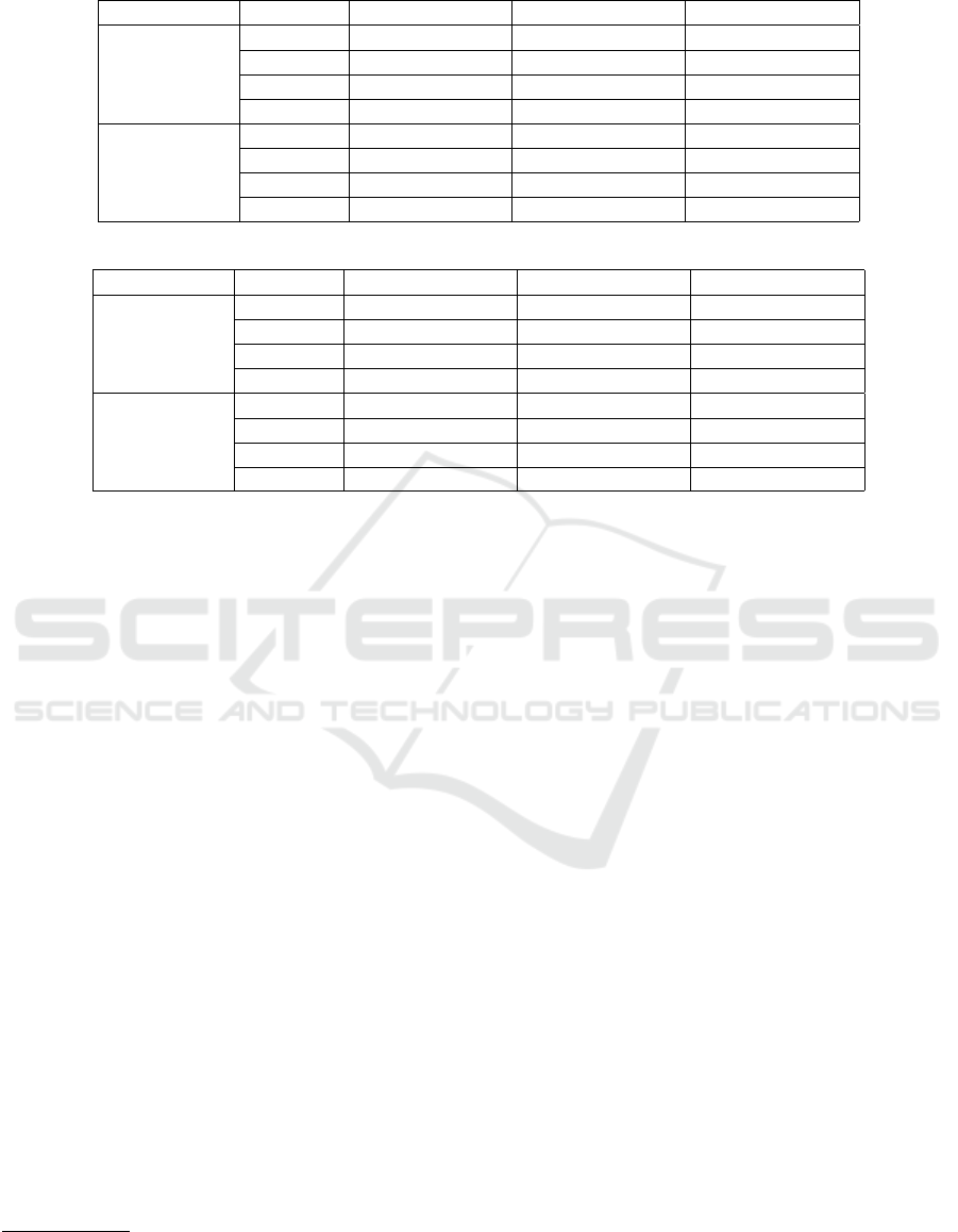
Table 2: MagNet and MultiMagNet’s performance on MNIST dataset for 40 experiments.

Defense Attack ACC (µ - σ) PPV (µ - σ) NPV (µ - σ)

MagNet

FGSM 99.90% - 0.37% 99.81% - 0.70% 100.00% - 0.00%

BIM 99.90% - 0.30% 99.81% - 0.58% 100.00% - 0.00%

DeepFool 96.43% - 2.20% 92.83% - 4.30% 100.00% - 0.00%

CW 56.00% - 5.17% 94.84% - 2.99% 27.54% - 7.85%

MultiMagNet

FGSM 99.92% - 0.26% 99.85% - 0.51% 100.00% - 0.00%

BIM 99.92% - 0.26% 99.85% - 0.54% 100.00% - 0.00%

DeepFool 96.47% - 1.48% 92.90% - 3.08% 100.00% - 0.00%

CW 61.10% - 5.74% 45.99% - 22.23% 75.24% - 15.25%

Table 3: MagNet and MultiMagNet’s performance on CIFAR-10 dataset for 40 experiments.

Defense Attack ACC (µ - σ) PPV (µ - σ) NPV (µ - σ)

MagNet

FGSM 58.43% - 5.56% 90.15% - 4.07% 26.35% - 8.51%

BIM 77.72% - 3.91% 88.98% - 3.50% 69.75% - 6.42%

DeepFool 71.88% - 21.18% 93.03% - 2.73% 49.93% - 42.93%

CW 66.55% - 6.53% 98.43% - 4.40% 45.20% - 10.95%

MultiMagNet

FGSM 65.88% - 4.48% 67.13% - 12.64% 65.06% - 13.22%

BIM 79.38% - 6.13% 66.57% - 15.42% 89.11% - 6.95%

DeepFool 90.25% - 4.66% 80.67% - 9.22% 99.86% - 0.69%

CW 68.95% - 4.45% 48.82% - 8.80% 84.31% - 5.96%

5.3 Prototype

The MultiMagNet prototype has been developed in

Python, by using the following frameworks: (i) Ten-

sorﬂow, (ii) Keras, (iii) SciKit-Learn, (iv) NumPy and

(v) Scipy. All the source code, including the archi-

tectures and parameters deﬁned for the autoencoders

and applications classiﬁers are available for consulta-

tion and/or download

. The adversarial images used

in the experiments are also available for download

All the experiments have been conducted on a sin-

gle machine with the following setup: CPU i7 3770,

16GB RAM and a GPU GTX 1060 with 1280 CUDA

cores.

5.4 Results

It has been performed 40 experiments on the respec-

tive D sets of MNIST and CIFAR-10 datasets. For ev-

ery 100 input images (once D set has a total of 4,000

images), a new ensemble R containing n different au-

toencoders has been formed, where n ∈ {3,5,7, 9} for

MultiMagNet and n = 1 for MagNet. It is worth re-

membering that n must be an odd number to avoid

ties. Tables 2 and 3 show the results of the mean µ and

standard deviation σ obtained by MagNet and Multi-

MagNet (based on 40 experiments) using the metrics

deﬁned by Equation 9.

https://github.com/gabrielrmachado/MultiMagNet

https://drive.google.com/open?id=

1l5KHwpbWLLgcv34AGUF3Fq3z3fuXV22z

When analyzing the results of MagNet and Mul-

tiMagNet included in Tables 2 and 3, it becomes

clearer that MultiMagNet has presented better per-

formance on the metric NPV than MagNet for all

attack algorithms on both datasets. The good per-

formance presented by MultiMagNet on NPV met-

ric indicates its better ability to detect adversarial im-

ages, which is priority in most security-critical appli-

cations. However, by analyzing Table 4, it can be

noticed that the adoption of the minimum threshold

approach (minTA) in most of attack scenarios may

explain the increase of the NPV metric, mainly be-

cause the minTA metric assigns the smallest com-

puted threshold for all the n chosen autoencoders. In

addition to the minimum threshold approach, the false

positive rate hyperparameter t

f p

may have also inﬂu-

enced in the fall of PPV metric, since smaller values

of t

f p

than the ones in Table 4 have produced an in-

crease in the PPV metric to the detriment of the NPV

metric. Nevertheless, the fall presented by MultiMag-

Net in the PPV metric is justiﬁable, due to the fact that

it has obtained greater accuracy than MagNet on both

datasets, before all the four evaluated attacks, reach-

ing differences up to 18.37 percentage points. Such

comparison points to the validation of the hypothesis

defended by this work.

Regarding the Table 6, which shows how strong

each attack was on leading F to misclassiﬁcation, it

is worth mentioning that, although the CW attack is

the state-of-the-art in generating adversarial images,

on MNIST dataset it has not been the attack algo-

MultiMagNet: A Non-deterministic Approach based on the Formation of Ensembles for Defending Against Adversarial Images

315

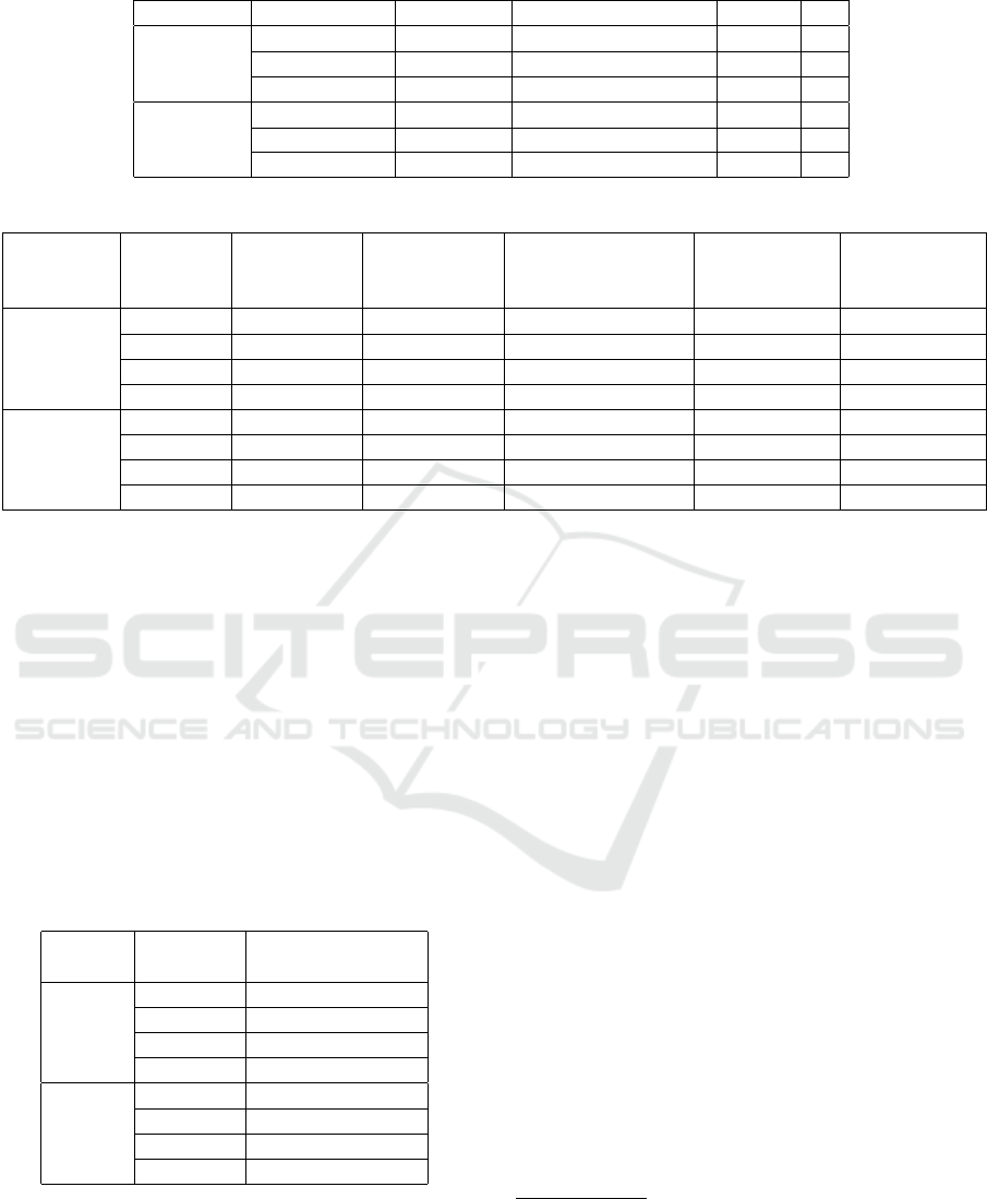
Table 4: MultiMagNet’s hyperparameters deﬁned for each attack algorithm.

Dataset Attack Drop Rate Threshold Approach Metric K

MNIST

FGSM - BIM 0.001 MTA RE -

DeepFool 0.07 MTA JSD 1

CW 0.05 minMTA RE -

CIFAR-10

FGSM - BIM 0.1 minMTA JSD 15

DeepFool 0.07 minMTA JSD 1

CW 0.07 minMTA JSD 5

Table 5: Accuracies obtained by the application classiﬁer F on D set when evaluated in ﬁve different scenarios.

Dataset Attack

No defense

(µ - σ) (%)

MagNet only

(µ - σ) (%)

MultiMagNet only

(µ - σ) (%)

MagNet

and Reformer

(µ - σ) (%)

MultiMagNet

and Reformer

(µ - σ) (%)

MNIST

FGSM 79.53 - 4.52 99.37 - 1.11 99.46 - 1.06 98.98 - 1.75 99.17 - 1.41

BIM 81.45 - 3.29 99.40 - 1.03 99.49 - 1.20 99.16 - 1.18 99.19 - 1.61

DeepFool 50.00 - 5.38 99.95 - 0.31 99.95 - 0.31 99.90 - 0.46 99.95 - 0.31

CW 81.60 - 4.33 92.92 - 3.21 98.71 - 1.72 96.19 - 2.20 98.89 - 1.36

CIFAR-10

FGSM 64.83 - 2.94 67.27 - 1.01 72.81 - 3.59 70.08 - 2.49 72.91 - 2.75

BIM 69.30 - 1.85 89.12 - 2.92 89.94 - 1.42 92.58 - 2.41 96.75 - 3.54

DeepFool 65.97 - 2.03 79.12 - 10.05 92.52 - 1.67 87.15 - 4.48 92.91 - 2.88

CW 47.03 - 1.29 59.14 - 3.29 71.86 - 5.74 60.08 - 3.27 72.36 - 5.22

rithm which fooled at most the application classiﬁer F

(when compared to DeepFool attack). This is mainly

due to two reasons: (i) CW is the attack which con-

tains the largest number of hyperparameters (see Ta-

ble 1); (ii) the MNIST images contain much less in-

formation on them (when compared to the CIFAR-10

images), what have proved to be more computation-

ally expansive to ﬁnd a set of hyperparameters for the

CW attack which could produce more harmful images

to F without increasing their amount of perturbation.

Nonetheless, according to Table 2, the adversarial im-

ages produced by CW attack on MNIST dataset have

been the most difﬁcult ones to be detected.

Table 6: Accuracies obtained by the application classiﬁer F

on D

atk

set, without any previous defense.

Dataset Attack

Accuracy D

atk

set

(no defense)

MNIST

FGSM 59.65%

BIM 63.50%

DeepFool 0.60%

CW 63.80%

CIFAR

FGSM 40.60%

BIM 49.55%

DeepFool 42.70%

CW 5.00%

Finally, in addition to the scenario depicted by

Table 6, the application classiﬁer F has been evalu-

ated in more ﬁve scenarios: (i) performance on D set

without any defense, (ii) performance on D set with

MagNet, (iii) performance on D set with MultiMag-

Net, (iv) performance on D set with MagNet and Re-

former

and (v) performance on D set with Multi-

MagNet and Reformer. It is important to highlight

that it has been also computed the mean µ and stan-

dard deviation σ of F’s accuracy in 40 experiments

for each scenario. The accuracies obtained by F for

all these scenarios are present in Table 5.

Although the presence of MagNet has provided

some sort of protection to F (when compared to the

results belonging to Scenario (i)), it becomes noto-

rious, by comparing the results in Table 5 related to

Scenarios (ii) and (iii), that MultiMagNet has also

overcome MagNet when the performance of F is

taken into account, thus providing to F a better pro-

tection than MagNet. It is also worth mentioning that

the Reformer step has had signiﬁcant importance on

improving even more the performance of F, as it can

be seen by the results related to Scenario (v). This

may be related to the fact that, even with the adoption

of an ensemble for detecting perturbations, few adver-

sarial images still might have been able to bypass the

MultiMagNet’s detection step and fool F. So, the Re-

formed step has behaved as an additional protection

to the application classiﬁer. Therefore, the results in

Tables 2, 3 and 5 emphasise that MultiMagNet has

been more effective than MagNet in detecting adver-

The word ”Reformer” refers to the Reform Image pro-

cess, as illustrated by Figure 4 and explained in Section

4.2.5.

It has been formed a new ensemble R for every 100

input images belonging to D set, in a way similar to the

experiments which produce the results in Tables 2 and 3.

ICEIS 2019 - 21st International Conference on Enterprise Information Systems

316

sarial images and protecting the application classiﬁer,

thus providing further signiﬁcant evidences that the

hypothesis raised by this work is true.

6 FINAL CONSIDERATIONS

In recent years, several work have demonstrated that

Deep Neural Networks are susceptible to be intention-

ally induced to misclassiﬁcation by adversarial im-

ages (i.e. images which contain perturbations, usu-

ally imperceptible to human eyes), fact that which

precludes the application of these learning algorithms

in several security-critical decision support systems

(Klarreich, 2016). Although various defenses have

been proposed against adversarial images, most of

them have already been bypassed by allowing the

attacker to easily map their inner behaviour. As a

means of reducing the behaviour predictability, a re-

search has aimed to create a non-deterministic detec-

tion method called MagNet (Meng and Chen, 2017).

However, recent studies reveal MagNet can also be

bypassed by adversarial images (Carlini and Wagner,

2017b).

Before this alarming scenario, the present work

has raised the hypothesis the insertion of multiple de-

fense components, randomly selected, in the detection

method can amplify the non-deterministic effect and

thus making the defense more robust than MagNet be-

fore different attack algorithms. Therefore, this work

has introduced MultiMagNet, a method for detect-

ing adversarial images which makes use of multiple

defense components (implemented as autoencoders),

selected at random and arranged in ensembles for de-

cision making. The experimental results performed

on images from MNIST and CIFAR-10 dataset point

to the veracity of the raised hypothesis, showing that

MultiMagNet has overcome MagNet (the MultiMag-

Net’s version which randomly chooses only one au-

toencoder) in most of the evaluated scenarios. In sum-

mary, the following main contributions of this work

are:

• The development of MultiMagNet, a non-

deterministic defense based of ensembles for de-

tecting adversarial images in decision support sys-

tems;

• The accomplishment of the ﬁrst

comparative

study with MagNet, in order to validate the hy-

pothesis raised by this work;

• The online availability of all the implementation

and needed resources for reproducing the experi-

ments.

Regarding the best of the authors’ knowledge.

For future work, it can be highlighted: (i) the

research of novel non-deterministic architectures for

detecting and classifying adversarial images, (ii) the

implementation of novel techiniques to automatically

deﬁne classiﬁcation thresholds, (iii) the adoption of

different techniques for preprocessing images.

ACKNOWLEDGMENTS

The present work has been conducted with the support

of the Coordenac¸

ao de Aperfeic¸oamento de Pessoal

de N

ıvel Superior - Brazil (CAPES) - Finacing Code

001.

REFERENCES

Bae, G., Lee, H., Son, S., Hwang, D., and Kim, J. (2018).

Secure and robust user authentication using partial ﬁn-

gerprint matching. In Consumer Electronics (ICCE),

2018 IEEE International Conference on, pages 1–6.

IEEE.

Carlini, N. and Wagner, D. (2017a). Adversarial Examples

Are Not Easily Detected: Bypassing Ten Detection

Methods. In 10th ACM Workshop on Artiﬁcial Intelli-

gence and Security, page 12, Dallas, TX.

Carlini, N. and Wagner, D. (2017b). Magnet and” ef-

ﬁcient defenses against adversarial attacks” are not

robust to adversarial examples. arXiv preprint

arXiv:1711.08478.

Carlini, N. and Wagner, D. (2017c). Towards evaluating the

robustness of neural networks. In 2017 IEEE Sym-

posium on Security and Privacy (SP), pages 39–57.

IEEE.

Derawi, M. O., Nickel, C., Bours, P., and Busch, C. (2010).

Unobtrusive user-authentication on mobile phones us-

ing biometric gait recognition. In Intelligent Informa-

tion Hiding and Multimedia Signal Processing (IIH-

MSP), 2010 Sixth International Conference on, pages

306–311. IEEE.

Ding, L., Fang, W., Luo, H., Love, P. E., Zhong, B., and

Ouyang, X. (2018). A deep hybrid learning model to

detect unsafe behavior: integrating convolution neural

networks and long short-term memory. Automation in

Construction, 86:118–124.

Gong, Z., Wang, W., and Ku, W.-S. (2017). Adversar-

ial and clean data are not twins. arXiv preprint

arXiv:1704.04960.

Goodfellow, I., Bengio, Y., and Courville, A. (2016). Deep

Learning. MIT Press. http://www.deeplearningbook.

org.

Goodfellow, I., Shlens, J., and Szegedy, C. (2015). Explain-

ing and harnessing adversarial examples. In Interna-

tional Conference on Learning Representations.

He, K., Zhang, X., Ren, S., and Sun, J. (2016). Deep Resid-

ual Learning for Image Recognition. In 2016 IEEE

MultiMagNet: A Non-deterministic Approach based on the Formation of Ensembles for Defending Against Adversarial Images

317

Conference on Computer Vision and Pattern Recogni-

tion (CVPR), pages 770–778. IEEE.

He, W., Wei, J., Chen, X., Carlini, N., and Song, D. (2017).

Adversarial Example Defenses: Ensembles of Weak

Defenses are not Strong. In 11th USENIX Workshop

on Offensive Technologies (WOOT’ 17), Vancouver,

CA.

Hendrycks, D. and Gimpel, K. (2017). Early methods for

detecting adversarial images. Workshop track -ICLR

2017.

Hu, J., Shen, L., and Sun, G. (2017). Squeeze-

and-excitation networks. arXiv preprint

arXiv:1709.01507.

Kannan, H., Kurakin, A., and Goodfellow, I. (2018). Adver-

sarial logit pairing. arXiv preprint arXiv:1803.06373.

Karpathy, A. (2014). What I learned from competing

against a ConvNet on Imagenet. Available at

http://karpathy.github.io/2014/09/02/what-i-learned-

from-competing-against-a-convnet-on-imagenet.

Accessed in September 02, 2018.

Klarreich, E. (2016). Learning securely. Communications

of the ACM, 59(11):12–14.

Krizhevsky, A. and Hinton, G. (2009). Learning multiple

layers of features from tiny images.

Kurakin, A., Goodfellow, I., and Bengio, S. (2016a). Adver-

sarial examples in the physical world. arXiv preprint

arXiv:1607.02533.

Kurakin, A., Goodfellow, I., and Bengio, S. (2016b). Ad-

versarial machine learning at scale. arXiv preprint

arXiv:1611.01236.

LeCun, Y., Bottou, L., Bengio, Y., and Haffner, P. (1998).

Gradient-based learning applied to document recogni-

tion. Proceedings of the IEEE, 86(11):2278–2324.

Madry, A., Makelov, A., Schmidt, L., Tsipras, D., and

Vladu, A. (2017). Towards deep learning mod-

els resistant to adversarial attacks. arXiv preprint

arXiv:1706.06083.

Meng, D. and Chen, H. (2017). Magnet: a two-pronged

defense against adversarial examples. In Proceedings

of the 2017 ACM SIGSAC Conference on Computer

and Communications Security, pages 135–147. ACM.

Metzen, J. H., Genewein, T., Fischer, V., and Bischoff, B.

(2017). On detecting adversarial perturbations. arXiv

preprint arXiv:1702.04267.

Moosavi-Dezfooli, S.-M., Fawzi, A., and Frossard, P.

(2016). Deepfool: a simple and accurate method to

fool deep neural networks. In Proceedings of the IEEE

Conference on Computer Vision and Pattern Recogni-

tion, pages 2574–2582.

Nicolae, M.-I., Sinn, M., Tran, M. N., Rawat, A., Wistuba,

M., Zantedeschi, V., Baracaldo, N., Chen, B., Ludwig,

H., Molloy, I., and Edwards, B. (2018). Adversarial

robustness toolbox v0.3.0. CoRR, 1807.01069.

Obermeyer, Z. and Emanuel, E. J. (2016). Predicting

the future — big data, machine learning, and clini-

cal medicine. The New England journal of medicine,

375(13):1216.

Papernot, N., McDaniel, P., Goodfellow, I., Jha, S., Celik,

Z. B., and Swami, A. (2017). Practical Black-Box At-

tacks against Machine Learning. In ACM Asia Con-

ference on Computer and Communications Security

(ASIACCS), pages 506–519.

Papernot, N., McDaniel, P., Jha, S., Fredrikson, M., Ce-

lik, Z. B., and Swami, A. (2016a). The limitations of

deep learning in adversarial settings. In Security and

Privacy (EuroS&P), 2016 IEEE European Symposium

on, pages 372–387. IEEE.

Papernot, N., McDaniel, P., Wu, X., Jha, S., and Swami,

A. (2016b). Distillation as a Defense to Adversar-

ial Perturbations Against Deep Neural Networks. In

Proceedings - 2016 IEEE Symposium on Security and

Privacy, SP 2016, pages 582–597.

Springenberg, J. T., Dosovitskiy, A., Brox, T., and Ried-

miller, M. (2014). Striving for simplicity: The all con-

volutional net. arXiv preprint arXiv:1412.6806.

Srivastava, S., Priyadarshini, J., Gopal, S., Gupta, S., and

Dayal, H. S. (2019). Optical character recognition

on bank cheques using 2d convolution neural network.

In Applications of Artiﬁcial Intelligence Techniques in

Engineering, pages 589–596. Springer.

Szegedy, C., Zaremba, W., Sutskever, I., Bruna, J., Erhan,

D., Goodfellow, I., and Fergus, R. (2013). Intriguing

properties of neural networks. In International Con-

ference on Learning Representations, pages 1–10.

Tolosana, R., Vera-Rodriguez, R., Fierrez, J., and Ortega-

Garcia, J. (2018). Exploring recurrent neural networks

for on-line handwritten signature biometrics. IEEE

Access, 6(5128-5138):1–7.

Xu, W., Evans, D., and Qi, Y. (2018). Feature squeez-

ing: Detecting adversarial examples in deep neural

networks. Network and Distributed Systems Security

Symposium (NDSS) 2018.

Zantedeschi, V., Nicolae, M.-I., and Rawat, A. (2017). Efﬁ-

cient defenses against adversarial attacks. In Proceed-

ings of the 10th ACM Workshop on Artiﬁcial Intelli-

gence and Security, pages 39–49. ACM.

ICEIS 2019 - 21st International Conference on Enterprise Information Systems

318