
Object Detection Probability for Highly Automated Vehicles:
An Analytical Sensor Model
Florian Alexander Schiegg
1,2
, Ignacio Llatser
2
and Thomas Michalke
3
1
Institute of Communications Technology, Leibniz University of Hannover, Appelstraße 9A, Hannover, Germany
2
Robert Bosch GmbH, Corporate Research, Robert-Bosch-Strasse 200, Hildesheim, Germany
3
Robert Bosch GmbH, Corporate Research, Robert-Bosch-Campus 1, Renningen, Germany
Keywords: Sensor Model, Object Detection, Advanced Driver Assistance Systems, Collective Perception, V2X,
Environmental Model, Highly Automated Driving, Cooperative Awareness.
Abstract: Modern advanced driver assistance systems (ADAS) increasingly depend on the information gathered by the
vehicle’s on-board sensors about its environment. It is thus of great interest to analyse the performance of
these sensor systems and its dependence on macroscopic traffic parameters. The work at hand aims at building
up an analytical model to estimate the number of objects contained in a vehicle’s environmental model. It
further considers the exchange of vehicle dynamics and sensor data by vehicle-to-vehicle (V2X)
communication to enhance the environmental awareness of the single vehicles. Finally, the proposed model
is used to quantify the improvement in the environmental model when complementing sensor measurements
with V2X communication.
1 INTRODUCTION
The increasing road traffic automation has come
along with the need for highly reliable environmental
models of the automated vehicle’s surroundings. In
order to be able to assist the driver or even take
decisions themselves, vehicles have to perceive their
surroundings and detect possible dangers and hazards
as precisely as possible.
To this end, the data recorded by the vehicle’s on-
board sensors, like video cameras, radars or LIDARs
is aggregated by making use of association algorithms
like the Joint Probabilistic Data Association (JPDA)
(Rezatofighi, et al., 2015) and subsequently filtered
and fused by algorithms such as Kalman or Particle
filters (Chen, 2003). All of these algorithms
sensitively depend on the accuracy of the processed
sensor data. The more data is available about an
object, the more precisely its current state may be
determined. Once a new object is detected and
validated this way, it is incorporated into the vehicle’s
environmental model. As long as the object stays
within the vehicle’s Field-of-View (FOV), it is kept
in the environmental model and its state is
periodically updated until it is no longer perceived for
a certain time.
However, one of the main limitations of current
on-board object detection sensors is the shadowing of
the FOV by obstacles and traffic objects in the
vicinity. To mitigate this impairment, Vehicle-to-
Everything (V2X) communication has been receiving
increasing interest lately. By sharing information of
their local environmental models with neighbouring
vehicles, V2X-capable vehicles are able to
significantly increase their knowledge about their
surroundings. The environmental model arising from
including V2X-Data into the local environmental
model (LEM) is commonly referred to as the global
environmental model (GEM). It not only allows to
substantially enhance the accuracy of the managed
data, but it may also include objects that are out of the
sensor’s Line-of-Sight (LOS) and thus not contained
within the LEM. Nevertheless, the GEM may still be
incomplete or even faulty. Hence, it is of great
importance for automated vehicles to be able to
estimate the accuracy of the environmental model at
the time they are facing a decision. Below a model is
derived analytically, that aims at determining the
number of objects known to the vehicle based on (i)
its own sensors and (ii) V2X communication with
vehicles in its vicinity. It is then demonstrated on the
example of a highway scenario.
Schiegg, F., Llatser, I. and Michalke, T.
Object Detection Probability for Highly Automated Vehicles: An Analytical Sensor Model.
DOI: 10.5220/0007767602230231
In Proceedings of the 5th International Conference on Vehicle Technology and Intelligent Transport Systems (VEHITS 2019), pages 223-231
ISBN: 978-989-758-374-2
Copyright
c
2019 by SCITEPRESS – Science and Technology Publications, Lda. All rights reserved
223

2 RELATED WORK
Considerable effort has been conducted in developing
more efficient object detection and tracking
algorithms for specific sensors or combinations of
them. An extensive overview is given by (Sivaraman,
2013). Empirical studies were performed for some of
these algorithms, to investigate the detection
probability given specific scenarios (Held, Levinson,
& Thrun, 2012). Geese et. al. (2018) recently
presented an approach to predict the performance of
an optical sensor in dependence of the environmental
conditions. Another approach is the detection and
tracking of moving objects (DATMO) based on
occupancy grids as presented, e.g. by Baig, Vu, &
Aycard (2009). However, to the best of the authors’
knowledge, no thorough theoretical analysis about the
number of detectable objects or the fraction of objects
contained in the LEM or the GEM has been
conducted so far.
The contribution of the present work is an
analytical model that allows estimating the absolute
and the relative amount of objects contained in both
LEM and GEM, in dependence of macroscopic
parameters, such as the linear vehicle density, and the
properties of road, vehicles and sensors.
3 VEHICLE PERCEPTION
In order to perceive their environment, automated
vehicles have to make use of all kinds of sensors.
While subsection 3.1 deals with the vehicle’s own on-
board sensors, subsection 3.2 introduces the concepts
of cooperative awareness and collective perception,
which allow utilizing the data of external sensors
shared through V2X communication.
3.1 On-board Sensors
The growing complexity of advanced driver
assistance systems (ADAS) is leading to an
increasing number of sensor-systems being installed
in nowadays’ vehicles. Fig. 1 shows some of them.
They can roughly be divided into four classes,
depending on their range: (i) ultra-short (up to 5 m):
e.g. ultrasound for parking assistance, (ii) short (~30
m): e.g. radar for blind spot detection, rear collision
warning or cross traffic alert, (iii) mid-range (~100
m): e.g. radar, LIDAR or video for surround view,
object detection, video-supported parking assistance,
traffic sign recognition, lane departure warning,
emergency braking or collision avoidance, and (iv)
long range (~200 m): radar e.g. for adaptive cruise
control or sheer-in assistance on a highway.
To ensure the functional safety of highly
automated vehicles, sensor redundancy for object
detection will be necessary, making sure the vehicle
is still able to deal with adverse environmental
conditions or even a sensor system falling out.
Figure 1: Vehicle sensors of ultra-short (grey), short
(green), medium (blue) and long range (red).
The LEM is essentially based on data registered by
the mid- and long-range sensors. To detect objects
that are further away, V2X communication is of great
use.
3.2 V2X Communication
The limited perception capabilities of on-board
sensors can be enhanced with V2X communication,
by means of cooperative awareness and collective
perception. Cooperative awareness consists of
vehicles transmitting data about their own state via
V2X communication, such as their current position,
speed and heading. This service is implemented by
the Cooperative Awareness Message (CAM) in
Europe and by the Basic Safety Message (BSM) in
the US. Collective perception (Günther, 2016) allows
cars to inform nearby vehicles of objects detected by
their own on-board sensors. The exchange of
Collective Perception Messages (CPM) enables
vehicles to perceive objects beyond their own
sensor’s range by looking through other vehicles’
“eyes”. The collective perception service is currently
considered for standardization by the European
Telecommunications Standards Institute (ETSI) in
order to ensure its interoperability among all
equipped vehicles.
4 ANALYTICAL MODEL
The quality of a highly automated vehicle’s
environmental model sensitively depends on the
fraction of objects it contains. It is thus necessary to
predict this quantity as accurately as possible. With
VEHITS 2019 - 5th International Conference on Vehicle Technology and Intelligent Transport Systems
224

this goal, an analytical model based on the
specifications of the vehicle dimensions, their on-
board sensors, the vehicle density and the scenario
characteristics is set up. The model should further
consider occlusion by other vehicles, which becomes
especially relevant at higher vehicle densities as
shown in the figure below, and V2X communication
among the vehicles.
Figure 2: Top view of a vehicle on a highway equipped with
a free-field sensor to detect traffic objects in its vicinity. The
NLOS section of the FOV (blue area) is indicated in cyan.
Finally, it would be desirable for the model to be as
independent of a concrete vehicle distribution as
possible, depending only on macroscopic parameters
such as the average vehicle velocity, density,
dimension and V2X penetration rate.
4.1 Objects in Field of View
The number of objects contained in a sensor’s FOV
(marked in blue in Fig. 2) is given by
(1)
where and
are the number of lanes within the
sensor’s FOV and the number of vehicles on lane
within the FOV respectively. The latter is defined by
the vehicle distribution
between the boundaries
and
(see example in Fig. 4) of the FOV on
line:
(2)
While the position of the analyzed vehicle, further
referred to as ego-vehicle, does have a significant
influence on the vehicle distribution on its own lane,
its effect on the distribution of vehicles on other lanes
is almost negligible (Filzek & Breuer, 2001). The
vehicle distribution can thus be assumed as isotropic
on each of these lanes and corresponds to their vehicle
densities
:
(3)
On the ego-lane however, the distribution is
characterized by the exact localization of the ego-
vehicle. The distribution function on the ego-lane is
thus composed of the distribution functions
of every vehicle on the ego-lane within the sensors
FOV
(4)
with the mean of
having to fulfill
〈
〉
!
(5)
While the distribution of the ego-vehicle equals a
simple Dirac delta function at the origin
(6)
the distributions of the neighbouring vehicles have
variance, skewedness and kurtosis that depend on the
mean vehicle density
and velocity
on the
ego-lane and follow the relation
,
,
,
,
(7)
where
and
are the mean vehicle length and
the inter-vehicle distance respectively. Numerous
studies have been conducted about the latter in the
past (Filzek & Breuer, 2001). By convolution, it is
then possible to recursively obtain the remaining
vehicle distribution functions:
∗
(8)
Fig. 3 shows a vehicle distribution around the ego-
vehicle. As expected,
(x) quickly tends towards
for 2 vehicles away from the ego-vehicle.
Figure 3: Vehicle distribution on ego-lane. The ego-vehicle
itself is represented by a Dirac-function at the origin.
Object Detection Probability for Highly Automated Vehicles: An Analytical Sensor Model
225
Putting together Eq. 1, 2 and 3 one obtains
(9)
≫
where
is the length of the lane segment of lane
within the FOV of the sensor and is the sensor’s
range. Fig 4 exemplarily shows
corresponding to
the distance between
and
. In general, for a
given sensor,
can be determined from the sensor’s
specifications. However, it can also easily be
determined by making use of sensor parameters, such
as its offset relative to the ego-vehicle’s front
axis
, its already introduced range and
the angles
and
delimiting its frustum.
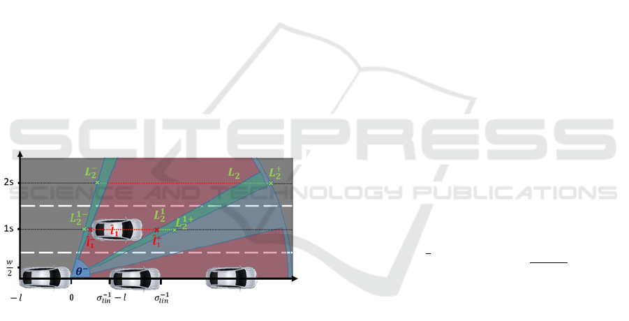
4.2 Objects in Line of Sight
Usually a relevant fraction of the vehicles in the
sensor’s FOV will be hidden behind closer objects.
These Non-Line-of-Sight (NLOS) segments are
depicted in red in the figure below (somewhat shorter
in range for a better visualization).
Figure 4: Schematic representation of a sensor’s Line-of-
Sight and Non-Line-of-Sight segments.
In analogy to Eq. 9, the number of objects within LOS
(green and blue segments in the figure above) is:
(10)
being the overall length of all lane sub-segments
on lane n that are in LOS.
Even though the vehicle may perceive further
objects on the ego-lane (e.g. due to misaligned
vehicles, different vehicle sizes or through the front
vehicle windows) the detection accuracy generally
will not be good enough to extract the necessary
information (e.g. to fill all the mandatory CPM object
fields). Thus, further detections on the ego-lane are
negligible. With this the expectancy value of
detectable objects
equivalents
capped on
one in both directions:
1
1
1
(11)
For instance, the second term of Eq. 10 may be
developed as follows
(12)
where
represents the fraction of visibility to lane
. The LOS fraction can take values from zero (if no
LOS is available) to one (when there are no occluding
vehicles). It is composed of the LOS-fractions of all
the lines between the ego-lane 0 and the target
lane and can be computed as:
(13)
Shadowing caused by vehicles on the ego-lane
reduces visibility towards the target lane. It may only
change the upper boundary of
. A geometric
analysis allows to calculate the expectancy value of
the last visible point on lane n
,
/
〈
〉
(14)
where and are the widths of the vehicle and the
lanes respectively. Eq. 10 can easily be resolved using
Eq. 4 and 5. Considering only vehicles on the ego-
lane, the LOS section of lane may thus be expressed
as:
,
min
,
,
,
(15)
At higher distances from the ego-lane, the number of
vehicles occluding the vision will increase. However,
objects on lanes in between may interfere in the LOS
only if they are placed between the sensor and its
theoretical visibility area on lane n (shown in green in
Fig. 4). Let’s define
as the portion of lane i where
vehicles could shadow lane n. As an example,
is
shown in Fig 4, comprising the segment from
to
. A simple geometrical analysis yields:
VEHITS 2019 - 5th International Conference on Vehicle Technology and Intelligent Transport Systems
226

(16)
The fraction of visibility on this line can now be
determined by
1
/
̅
(17)
where
/
stands for the number of vehicles on line
interfering the LOS to lane n and
̅
is their average
effective cross-section. Knowing that the x-position
relative to the ego-vehicle is not correlated (see
Section 4.1),
̅
can be computed as
̅
(18)
with
representing the projection of a vehicle at
position x on the center of lane i. For the sake of
simplicity, the sensor offset is omitted in Eq. 19 and
20, however it can easily be reincorporated
(19)
with the terms
/
and
/
.
Reincorporating this into Eq. 18 and solving the
integral yields:
2
0.5
(20)
Subsequently the number of shadowing vehicles on
the earlier lines
/
has to be determined for Eq. 17.
It can be computed by the recursive equation:
/
1
/
(21)
Due to the relation
/
the expectancy
value of detectable vehicles on lane can finally be
written as:
1
/
(22)
It should be noted that this is not equal to the number
of vehicles shadowing line , since only
/
of these vehicles will interfere the LOS to
line .
4.3 Objects Detected by V2X
Communication
Vehicles not detectable by on-board sensors can still
be detected via V2X communications, by means of
cooperative awareness and collective perception (see
Section 3.2). These services make it possible to
extend the own vehicle’s Local Environmental Model
(LEM) to an enhanced Global Environmental Model
(GEM), which includes vehicles detected by means
of V2X communication in addition to those detected
by the vehicle’s on-board sensors. The total number
of vehicles in the GEM can be expressed as:
(23)
Knowing that a car is detectable via on-board sensors
by
vehicles, one can compute the probability
that at least one of these vehicles is V2X-equipped,
and thus able to inform the ego-vehicle about the
detected car
1
1
(24)
where the +1 comes from the transmitting vehicle
sharing its own state through a CAM, a CPM or any
other V2X-message and being the V2X penetration
rate. With this, it is now possible to determine the
expectancy value of vehicles detected merely by V2X
communication:
1
1
(25)
5 RESULTS AND DISCUSSION
In this section, the theoretical model is demonstrated
and discussed on the example of a highly autonomous
vehicle on a straight highway segment. It is divided
into two sections, dealing with the LEM (Section 5.1)
and the GEM (Section 5.2) respectively. Different
performance metrics are analysed in dependence of
the vehicle density, the number of lanes, the V2X
penetration rate and the utilized sensor system. Due
Object Detection Probability for Highly Automated Vehicles: An Analytical Sensor Model
227
to its depreciable effect on the normalized vehicle
distribution (Fig. 3) and its strong correlation to the
vehicle density (Filzek & Breuer, 2001), the vehicle
velocity is not further investigated.
5.1 Local Environmental Model
Even though the presented analytical model already
builds on a number of simplifications, for
demonstration purposes a few more have to be
introduced. Below, they are presented together with the
necessary set of parameters:
Highly autonomous vehicles require a full
perception of their environment in order to act and
react according to it. Thus, a full surround view is
indispensable.
Sensor redundancy significantly increases the
reliability of the system. For this reason, full-
surround video, LIDAR, and radar systems, with
front and rear ranges of 100m (video), 120m
(LIDAR) and 180m (radar) are discussed.
Even though side sensors will have a much lower
range than their front and rear peers, it will be
sufficient to cover the full street width.
To reduce the number of variables a constant
vehicle density is presumed for the purposes of
this analysis.
The vehicle length and width are set to 4.4m and
1.8m respectively, corresponding to the average
dimensions of vehicles sold in Germany in 2018
(Centre for Automotive Research (CAR) of the
Duisburg-Essen University, 2018).
The lane width was set to 3.5m as defined in the
German RQ26, RQ33 and RQ10.5 highway
standards by the FGSV (1982).
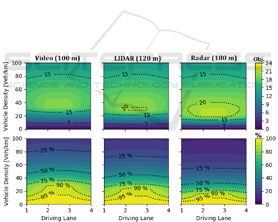
Fig. 5 shows the results of the postulated model for a)
the video-, b) the LIDAR-, and c) the radar-system on
a four-lane highway. The x- and y-axes of the upper
three plots represent the ego-lane and the vehicle
density respectively.
As could be expected, cars on the centre lanes
detect more vehicles than those on outer ones.
Moreover, the number of detectable objects reaches a
maximum for a certain vehicle density. The location of
this maximum further depends on the range of the
sensor system. Apparently, a higher range shifts the
maximum down to lower densities. This can easily be
explained, considering that the inter-vehicle distance
increases with decreasing vehicle density.
Figure 5: Expected object detections (above) and Environment Awareness Ratio (EAR, bellow) of a vehicle depending on its
actual driving lane on a 4-lane highway and the average linear vehicle density for different full surround sensor systems.
VEHITS 2019 - 5th International Conference on Vehicle Technology and Intelligent Transport Systems
228
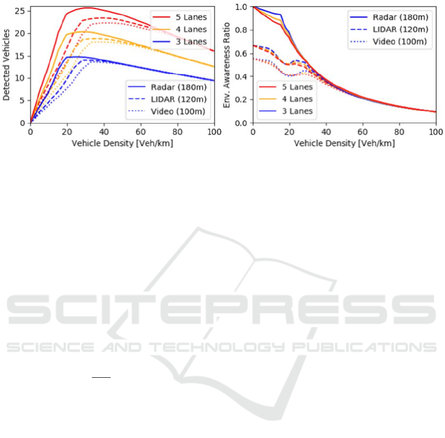
Figure 6: Vehicles in LOS (left) and Environmental Awareness Ratio (EAR, right) of a vehicle depending on the number of
highway-lanes and the vehicle density for full surround video, LIDAR and radar systems.
At low inter-vehicle distances, the number of
detected vehicles will not increase significantly with
increasing sensor range, since shadowing by cars in the
proximity dominates. However, at lower vehicle
densities, vehicles that are further away may also be
detected. The maxima are located at densities of
approximately 38 (video), 32 (LIDAR) and 21 (radar)
vehicles per kilometre. This corresponds to average
inter-vehicle distances of 22m, 27m and 41m
respectively, proving the direct correlation with the
range of the sensor system.
Besides the number of detectable vehicles, also
the Environmental Awareness Ratio (EAR) i.e. the
detection probability of an object within the FOV is
of great interest. It can be determined as follows:
EAR
(26)
The lower row of Fig. 5 shows the environmental
awareness ratio for a) the video-, b) LIDAR-, and c)
radar system. As can be seen, the number of
detectable objects decreases at lower densities,
however, the awareness ratio improves due to the lack
of shadowing vehicles in the vicinity. For this reason,
the EAR is essential to complement the number of
detectable objects.
To investigate the effect of the number of lanes on
the number of detectable objects, the latter was
determined for highways of 3, 4, and 5 lanes as an
average over each of their lanes for the three
investigated sensor systems (Fig. 6, left). It is worth
noticing that the maximal amount of detectable
vehicles always moves towards higher densities with
increasing number of lanes. Moreover, the previous
findings of the four-lane highway seem to hold
accordingly for the three- and five-lane highways.
Opposed to the EARs of Fig. 5, which were normed
on the ranges of each sensor system, the EARs in Fig.
6 (right) take the range of the radar system as
reference. This allows to directly compare the
performances of the three sensor systems. As was to
be expected, the radar system clearly outperforms the
radar and video systems at vehicle densities of up to
20 vehicles per kilometre due to its higher range.
However, in the region between 20 and 40 vehicles
per kilometre the performance gap closes quickly,
and almost fully vanishes for densities over 40
vehicles per kilometre. Another interesting, yet
expectable finding is that the number of lanes has a
much smaller effect on the EAR. The addition of
further lanes only leads to a slight deterioration of the
vehicle’s environmental awareness. Finally, the fast
drop in EAR with the vehicle density down to around
10% at a density of 100 vehicles per kilometre clearly
emphasises the need for an enhancement of the LEM.
5.2 Global Environmental Model
To investigate the GEM, further assumptions and
simplifications are made:
The channel capacity is expected to be high
enough to avoid channel congestion.
The communication range is assumed high
enough to cover double the sensor range.
Considering current technologies, e.g. LTE-
V2X, IEEE 802.11p and the upcoming 5G-V2X,
the communication range should not be a
limiting factor on a highway scenario (Molina-
Masegosa, 2017)
The number of transmitted objects per CPM is
limited to 20 to control the message size.
Fig. 7 shows the results for V2X penetration rates of
0% (
) to 100% (
for a five-
Object Detection Probability for Highly Automated Vehicles: An Analytical Sensor Model
229
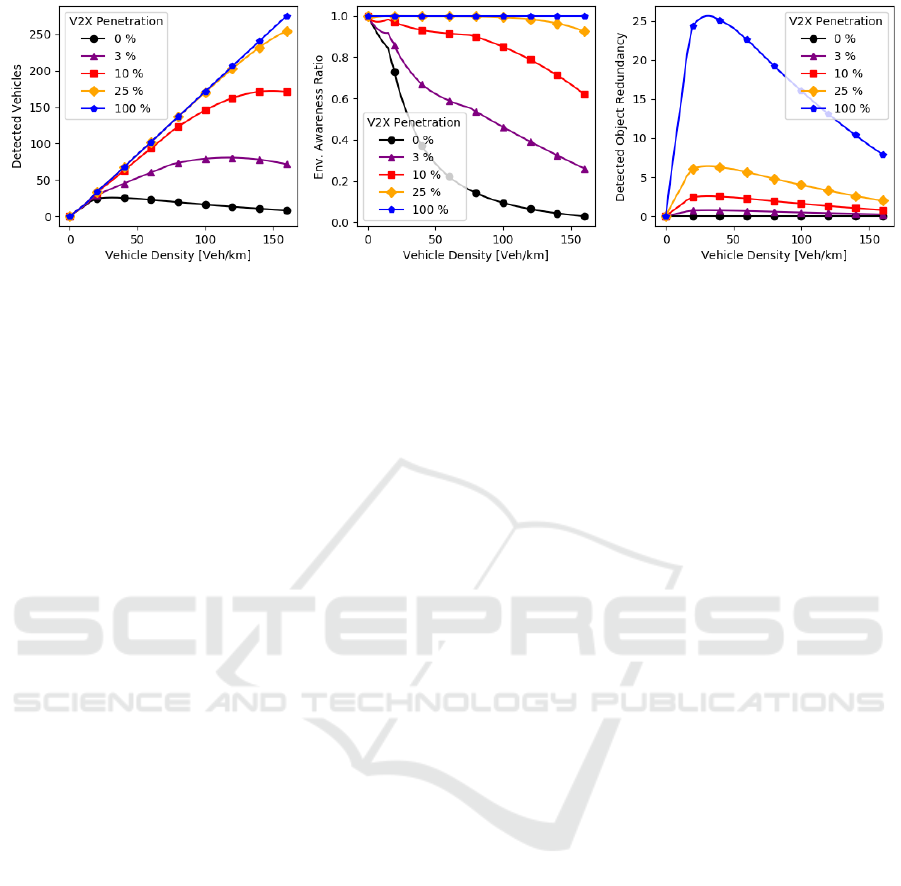
Figure 7: Expected number of vehicles contained in a vehicle’s GEM (left), Environmental Awareness Ratio (EAR, middle),
and Detected Object Redundancy (DOR, right) depending on the V2X penetration rate for a five-lane highway (Radar).
lane highway scenario. Clearly, collective perception
significantly increases the number of detected objects
(left) and hence the environmental awareness
(middle) already at penetration rates of φ3
10%. Only at very small inter-vehicle distances of
around 2.5m (140Veh/km) the EAR decreases
to ~75% and ~96% for φ10% and φ25%
respectively, making higher penetration rates
necessary. However, higher penetration rates also
increase the Detected Object Redundancy (DOR,
Fig.7, right). While a penetration rate of φ10%
implies an expected detection redundancy of at most
3 objects for an EAR of at least 75%, the DOR
increases up to 7 and27 for penetration rates of φ
25% and φ100% respectively. Specially the
increase from φ25% to φ100% brings low
profit (∆EAR4%) at a high price (400% more
transmitted data), suggesting the need for regulation
mechanisms at higher V2X penetration rates.
6 CONCLUSION
The present work introduced an analytical model to
determine the number of vehicles within the FOV of
a sensor or a complete sensor system and the
respective LOS fraction. The latter is important to
estimate the quality of the LEM. It was found, that the
environmental awareness ratio suffers a significant
drop at denser traffic scenarios, making the exchange
of data through V2X communication necessary. The
integration of V2X services, such as cooperative
awareness and collective perception, led to a
significant enhancement of the environmental
awareness already at very low V2X penetration rates.
Higher penetration rates further increased the EAR;
however, the gain was small in comparison to the rise
in transmitted data.
The model builds a good analytical basis, not only
for the better understanding of current and future
sensor systems, but also for the development of V2X
services like the CPM and the corresponding
congestion control mechanisms.
REFERENCES
Baig, Q., Vu, T.-D., and Aycard, O. (2009). Online
localization and mapping with moving objects
detection in dynamic outdoor environments. IEEE 5th
International Conference on Intelligent Computer
Communication and Processing (pp. 401-408). IEEE.
Centre for Automotive Research (CAR) of the Duisburg-
Essen University. (2018, May 07). WACHSTUM - Die
Autos werden immer dicker. Der Standard.
Chen, Z. (2003). Bayesian Filtering: From Kalman Filters
to Particle Filters, and Beyond. Statistics, 182(1), 1-69.
Filzek, B., and Breuer, B. (2001). Distance behavior on
motorways with regard to active safety ~ A comparison
between adaptive-cruise-control (ACC) and driver.
SAE Technical Paper (No. 2001-06-0066).
Forschungsgesellschaft für Straßen- und Verkehrswesen
(FGSV). (1982). Richtlinien für die Anlage von
Straßen: (RAS) / Forschungs-gesellschaft für Straßen-
und Verkehrswesen, Arbeitsgruppe Straßenentwurf;
Teil (RAS-Q): Querschnitte. Köln:
Forschungsgesellschaft für Straßen- und
Verkehrswesen, Vol. 295.
Geese, M., Ulrich, S., and Alfredo, P. (2018). Detection
Probabilities: Performance Prediction for Sensors of
Autonomous Vehicles. Electronic Imaging 2018 (17),
1-14.
Günther, H. J. (2016). Realizing collective perception in a
vehicle. Vehicular Networking Conference (VNC) (pp.
1-8). IEEE.
Held, D., Levinson, J., and Thrun, S. (2012). A probabilistic
framework for car detection in images using context
and scale. In Robotics and Automation (ICRA) (pp.
1628-1634). IEEE International Conference.
VEHITS 2019 - 5th International Conference on Vehicle Technology and Intelligent Transport Systems
230

Molina-Masegosa, R. and. (2017). LTE-V for sidelink 5G
V2X vehicular communications: a new 5G technology
for short-range vehicle-to-everything communications.
IEEE Vehicular Technology Magazine 12(4) (pp. 30-
39). IEEE.
Rezatofighi, S. H., Milan, A., Zhang, Z., Shi, Q., Dick, A.,
and Reid, I. (2015). Joint probabilistic data association
revisited. IEEE International Conference on Computer
Vision (ICCV) (pp. 3047-3055). IEEE.
Sivaraman, S. and. (2013). Looking at vehicles on the road:
A survey of vision-based vehicle detection, tracking,
and behavior analysis. IEEE Trans-actions on
Intelligent Transportation Systems, 14(4) (pp. 1773-
1795). IEEE.
Object Detection Probability for Highly Automated Vehicles: An Analytical Sensor Model
231
