Balancing Control of a Self-driving Bicycle
T. J. Yeh, Hao-Tien Lu and Po-Hsuan Tseng
Department of Power Mechanical Engineering, National Tsing Hua University, Hsinchu 30013, Taiwan
Keywords:
Balancing Control, Bicycle, Convex Combination, Linear Matrix Inequality.
Abstract:
In this research, a self-driving bicycle is constructed and the balancing control using the handlebar is stud-
ied. The controller is designed based on a model which characterizes the bicycle’s lateral dynamics under
speed variations. As the model can be decomposed into a convex combination of four linear subsystems
with time-varying coefficients, the proposed controller also consists of a convex combination of four linear,
full-state feedback controllers. It is proved that if the full-state feedback controllers satisfy a set of linear
matrix inequalities, the bicycle can maintain its lateral stability regardless of speed changes. Both simulations
and experiments verify that the proposed controller can achieve robust balancing performance under various
operating conditions.
1 INTRODUCTION
As the least expensive means of wheeled transporta-
tion, bicycles are widely used for many activities such
as commute, sport, recreation and so on. Bicycles
are considered to be environmentally friendly because
they can reduce the traffic congestion and air pollu-
tion in urban areas. The recent introduction of elec-
tric bicycles can further enhance the range and mo-
bility of bicycles. From system dynamics perspec-
tive, bicycles are in the category of wheeled-inverted-
pendulum vehicles and exhibit interesting dynamic
behavior. Modeling, analysis, and control of bicycles
thus have attracted significant attention in research
community ever since they were invented.
Whipple(Whipple, 1899) pioneered his work on
bicycle modeling by firstly deriving the equations of
motion of the bicycle. His model, which consid-
ered the bicycle as an assembly of four rigid bod-
ies, is both rigorous and complete. However, it is
not suitable for control system studies because it is
is highly nonlinear and complex. For this reason,
several simplified models have been proposed. For
example, Sharp(Sharp, 1971) used a four-degree-of-
freedom model to analyze the forward stability of
a bicycle. Lowell et.al.(Lowell and McKel, 1982)
lumped the whole bicycle as a point mass and used an
inverted pendulum to describe the lateral dynamics.
K. J. Astrom(Astrom et al., 2005) further augmented
the inverted pendulum model by incorporating steer-
ing angle as the input to the front fork assembly. In
(Meijaard et al., 2007), a benchmark model for the bi-
cycle was presented by Meijaard et. al.. This model,
which is a linear time-varying system parameterized
by the bicycle speed, is obtained by linearizing the
motion equations for small perturbations around the
constant-speed straight-ahead upright trajectory.
Regarding the control studies for bicycles, the re-
cent advances in digital computers, sensor and ac-
tuator technologies have drawn significant research
interests on developing self-balancing bicycles. For
instance, Beznos et al.(Beznos et al., 1998) con-
trolled the precession of the gyroscopes to gener-
ate a gyroscopic torque to counteract the destabiliz-
ing gravitational torque so as to balance a bicycle.
In (Cerone et al., 2010), the authors exploited the
linear-parameter-varying (LPV) nature of the bicycle
model proposed in (Meijaard et al., 2007) to design
a control system that automatically balances a rid-
erless bicycle in the upright position. Their control
problem is formulated as the design of an LPV state-
feedback controller that guarantees stability when the
speed varies within a given range and its derivative
is bounded. While the steering torque is treated as
the control input in (Cerone et al., 2010), Tanaka and
Murakami(Tanaka and Murakami, 2004) applied PD
control to modulate the steering angle to stabilize the
roll motion of the bicycle. In (Huang et al., 2017), the
authors developed a miniaturized humanoid robot to
ride and pedal a bicycle of comparable size. The robot
balances and steers the bicycle via controlling the an-
gle of the handlebar. The controller, which is de-
signed based-on a constant-speed bicycle model, can
automatically counteract the mass imbalance in the
34
Yeh, T., Lu, H. and Tseng, P.
Balancing Control of a Self-driving Bicycle.
DOI: 10.5220/0007810600340041
In Proceedings of the 16th International Conference on Informatics in Control, Automation and Robotics (ICINCO 2019), pages 34-41
ISBN: 978-989-758-380-3
Copyright
c
 2019 by SCITEPRESS – Science and Technology Publications, Lda. All rights reser ved

robot-bicycle system and allow it to perform straight-
line steering and cornering.
In this research, balancing control of a real-size,
self-driving bicycle is studied. The model adopted
here for controller design considers speed variations
and thus can be characterized as an LPV system as in
(Meijaard et al., 2007). However, in stead of solving a
infinite family of linear matrix inequalities (LMI’s) as
in the reference, the model is converted into a special
format so that only a small number of LMI needed
to be solved to devise the controller for robust per-
formance under speed variations. The paper is orga-
nized as follows: A model that describes the speed-
dependent lateral dynamics of the bicycle is given in
Section II. Section III shows how the dynamic model
can be converted into a tractable form so as to conduct
robust balancing control design against speed varia-
tions . The performance of the control system is ver-
ified numerically in Section IV. Section V describes
the hardware setup of the self-driving bicycle and per-
forms experimental validation on the control perfor-
mance. Finally, conclusions are given in Section VI.
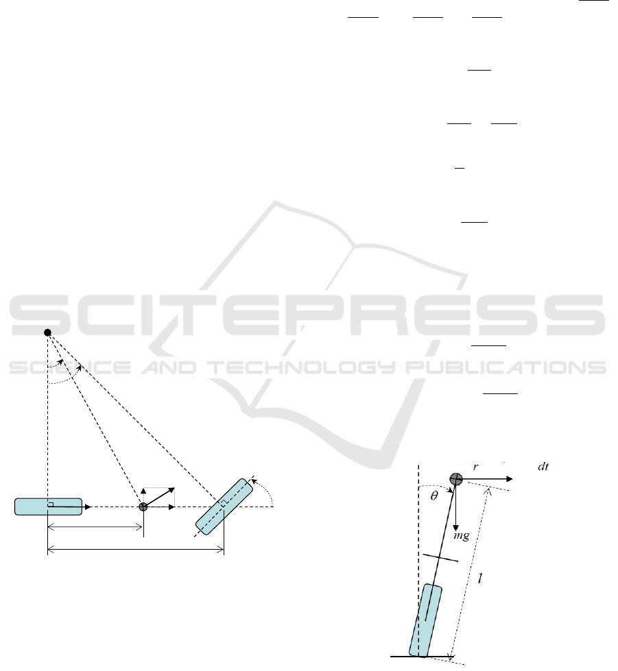
2 MODELING OF THE LATERAL
DYNAMICS
η
γ
η
y
v
r
O
a
b
c
O
g
O
r
0
r
f
O
0
v
x
v
v
Figure 1: Top view of a bicycle.
This section derives a model that describes the lat-
eral dynamics of a bicycle. The modeling approach
here is adopted from (Huang et al., 2017). To begin
with, the kinematic relations among crucial motion
variables are analyzed.
2.1 Kinematic Analysis
Fig. 1 shows the top view of a bicycle in which O
g
is
the center of gravity (COG) of the bicycle, O
f
is the
center of the front wheel, and O
r
is the center of the
rear wheel. Assume that the rear wheel is driven with
speed v
0
and the front wheel is steered with a direc-
tional angle η. Driving and steering actions make the
bicycle turn with respect to an instantaneous center of
rotation O
c
. Under the no-slip condition, O
c
is the in-
tersection of the two extension lines respectively from
the axles of the front and rear wheels. Let a = O
r
O
g
,
b = O
r
O
f
, r
0
= O
c
O
r
, r = O
c
O
g
, and γ = ∠O
r
O
c
O
g
,
so the following trigonometric relations hold:
r =
a
sinγ
, (1)
and
r
0
=
a
tanγ
=
b
tanη
. (2)
Notice that the yaw rate of the bicycle, which is de-
noted by
˙
φ, is equal to
v
0
r
0
. From the second equality
in (2),
˙
φ can be written as
˙
φ =
tanη
b
v
0
. (3)
Let v be the magnitude of the bicycle’s velocity at
the COG O
g
, and v
x
and v
y
be the components of the
velocity along and perpendicular to the bicycle body.
Since the bicycle body is rigid, we have v
x
= v
0
, and
v and v
y
are related to v
0
respectively by
v = r
˙
φ =
atanη
bsin γ
v
0
, (4)
and
v
y
= vsin γ =
atan η
b
v
0
. (5)
2.2 Dynamic Analysis
Figure 2: Frontal view of a bicycle.
In the the frontal view shown in Fig. 2, the bicycle
is modeled as an inverted pendulum whose mass m
is concentrated at the COG. The COG is located at
Balancing Control of a Self-driving Bicycle
35

a distance of l from the ground contact point with a
roll angle θ. Notice that the inverted pendulum sys-
tem in Fig. 2 may not be in an inertia frame when
the bicycle is in motion. Therefore, in addition to the
gravitational force, one also has to consider the inertia
force m
dv
y
dt
and the centrifugal force m
v
2
r
cosγ acting
on COG when deriving the dynamic equation. Apply-
ing Newton’s law and substituting the expressions of
v and v
y
in (4) and (5), the lateral dynamics is derived
as:
m`
2
¨
θ = m`cos θ(
v
2
r
cosγ +
dv
y
dt
) + mg` sin θ
= m`cos θ(
v
2
0
b
tanη +
av
0
sec
2
η
b
˙
η (6)
+
atan η
b
˙v
0
) + mg` sin θ
in which the second equality also utilizes the relation
tanγ =
a
b
tanη inferred from (2).
When both the the directional angle η and the roll
angle θ are small, the nonlinear dynamics in (6) can
be further linearized as
m`
2
¨
θ ≈ m`

(
v
2
0
b
+
a ˙v
0
b
)η +
av
0
b
˙
η

+ mg`θ (7)
It should be noted that the directional change of the
front wheel is due to the vertical projection of the ro-
tation of the steering handlebar via the caster angle
of the front fork assembly (The reader can refer to
(Tanaka and Murakami, 2004) for the graphical def-
inition of the caster angle.). Denoting the steering
angle of the handlebar by δ and the caster angle by
ε
0
, the directional angle η can be expressed as
η = sinε
0
· δ. (8)
Substituting the above expression into (7) yields
m`
2
¨
θ = m`
sinε
0
b
h
(v
2
0
+ a ˙v
0
)δ + av
0
˙
δ
i
+ mg`θ, (9)
or
¨
θ −
g
`
θ =
asin ε
0
v
0
b`

˙
δ + (
v
0
a
+
˙v
0
v
0
)δ

(10)
2.3 A State-space Model for Control
Design
According to (10), the open-loop system is unstable
due to the inverted pendulum mode which contains
an unstable pole at
q
g
`
. As a result, feedback con-
trol is needed to modulate the steering angle to stabi-
lize/balance the bicycle. For control design purposes,
we first convert (10) into a state-space form by defin-
ing the state vector x as

θ
˙
θ δ

T
and a new con-
trol input as
u =
˙
δ + (
v
0
a
+
˙v
0
v
0
)δ, (11)
and the state equation of the linearized lateral dynam-
ics of the bicycle is thus given as
˙
x = Ax + Bu, (12)
where A =


0 1 0
g
`
0 0
0 0 −
v
0
a
−
˙v
0
v
0


, B =


0
asinε
0
v
0
b`
1


.
The major challenge in the feedback control design
is that the presence of v
0
and ˙v
0
in the A and B ma-
trices makes the system dynamics time-varying when
the bicycle experiences speed changes. To facilitate
control design for the time-varying system, we as-
sume that the bounds for v
0
and
˙v
0
v
0
are known, or
(v
0
)
min
≤ v
0
≤ (v
0
)
max
and

˙v
0
v
0

min
≤
˙v
0
v
0
≤

˙v
0
v
0

max
where (v
0
)
min
and (v
0
)
max
are respectively the lower
bound and upper bound for v
0
and

˙v
0
v
0

min
, and

˙v
0
v
0

max
are respectively the lower bound and upper
bound for
˙v
0
v
0
.
Next we define two parameters α and β to repre-
sent the normalized values for v
0
and
˙v
0
v
0
respectively
as
α =
v
0
− (v
0
)
min
(v
0
)
max
− (v
0
)
min
, (13)
β =
˙v
0
/ ˙v
0
− ( ˙v
0
/ ˙v
0
)
min
( ˙v
0
/ ˙v
0
)
max
− ( ˙v
0
/ ˙v
0
)
min
(14)
in which 0 ≤ α,β ≤ 1. When v
0
and
˙v
0
v
0
in (12) are
replaced by α and β respectively, it can be derived
that
˙
x = A
0
x + B
0
u + αA
α
x + αB
α
u + βA
β
x (15)
where A
0
=



0 1 0
g
`
0 0
0 0 −
(v
0
)
min
a
−

˙v
0
v
0

min



, B
0
=


0
asinε
0
v
0
b`
1


, A
α
=


0 0 0
0 0 0
0 0 −
(v
0
)
max
−(v
0
)
min
a


,
B
α
=


0
asin ε
0
b`
((v
0
)
max
− (v
0
)
min
)
0


, and A
β
=


0 0 0
0 0 0
0 0 −(( ˙v
0
/ ˙v
0
)
max
− ( ˙v
0
/ ˙v
0
)
min
)


.
3 ROBUST BALANCING
CONTROL DESIGN
Given the transformed dynamic model in (15), the
control target is to devise a control law for u so as
ICINCO 2019 - 16th International Conference on Informatics in Control, Automation and Robotics
36

to robustly regulate the state x under the bounded and
time-varying parameters α and β. The control prob-
lem is solved by firstly converting the model into a
so-called “polytopic form”(Zak, 2003) as
˙
x =
4
∑
k=1
ρ
k
(t)(A
k
x+B
k
u) (16)
in which (15) is expressed as a linear combination of
four linear systems with system matrices A
(.)
and B
(.)
.
The derivation of the polytopic form and the defini-
tions of A
(.)
, B
(.)
, and ρ
(.)
are depicted in the follow-
ing lemma.
Lemma. The dynamic model in (15) can be trans-
formed into the polytopic form in (16) with
ρ
1
(t) = (1 − α) (1 − β) (17)
ρ
2
(t) = α(1 − β) (18)
ρ
3
(t) = (1 − α) β (19)
ρ
4
(t) = αβ, (20)
and
A
1
= A
0
, B
1
= B
0
,
A
2
= A
0
+ A
α
, B
2
= B
0
+ B
α
A
3
= A
0
+ A
β
, B
3
= B
0
A
4
= A
0
+ A
α
+ A
β
, B
4
= B
0
+ B
α
.
Proof. Because the definitions of ρ
(.)
in (17)-(20)
lead to ρ
2
+ ρ
4
= α, ρ
3
+ ρ
4
= β, and
∑
4
k=1
ρ
k
= 1,
(15) can be rewritten as
˙
x =
4
∑
k=1
ρ
k
!
(A
0
x + B
0
u)
+ (ρ
2
+ ρ
4
)(A
α
x + B
α
u)
+ (ρ
3
+ ρ
4
)A
β
x. (21)
By regrouping the above equation in the form of (16),
one can prove that A
k
’s and B
k
’s should satisfy the
expressions in the lemma.
Notice that the linear combination in (16) is con-
vex that in addition to
∑
4
k=1
ρ
k
= 1, the time-varying
coefficients ρ
k
(t)’s all fall between 0 and 1 due to
0 ≤ α, β ≤ 1. Models in this form are commonly re-
ferred as Takagi-Sugeno-Kang (TSK) fuzzy models.
In the fuzzy control research, TSK models have been
used extensively to design stabilizing controllers for
nonlinear systems. In this study, we adopt a simi-
lar control structure as the fuzzy full-state feedback
law(Zak, 2003) for the TSK models to stabilize the
lateral dynamics of the bicycle under speed variations.
The controller is a convex combination of four linear,
full-state feedback controllers with the same convex
coefficients as the plant model in (16):
u =
4
∑
j=1
ρ
j
K
j
x, (22)
where K
j
’s are feedback gain matrices. The associ-
ated closed-loop dynamics is given by
˙
x =
4
∑
k=1
4
∑
j=1
ρ
k
ρ
j
(A
k
+ B
k
K
j
)x (23)
The following theorem provides a synthesis
method for computing the stabilizing gain matrices
K
j
’s.
Theorem. Given the polytopic system in (16) with the
control law in (22), for W = W
T
> 0 ∈ R
4×4
and λ >
0 ∈ R, if there exist Y
1
,Y
2
,Y
3
,Y
4
∈ R
2×4
satisfying
the following linear matrix inequalities (LMI’s):
(A
k
+A
j
)W + W (A
k
+ A
j
)
T
+

Y
T
j
B
T
k
+B
k
Y
j
) +

Y
T
k
B
T
j
+ B
j
Y
k

+ 4λW ≤ 0 (24)
for all k ≤ j, k, j ∈
{
1,2, 3,4
}
, then the closed-loop
system is globally exponentially stable by setting
K
j
= Y
j
W
−1
, j = 1 ∼ 4. (25)
Furthermore,
k
x(t)
k
2
is bounded by
C
k
x(0)
k
2
e
−λt
for some finite constant C.
Proof. For the Lyapunov function defined by V (x) =
1
2
x
T
Px where P = W
−1
, its time derivative along the
closed-loop system trajectory (23) is
˙
V =
4
∑
k=1
4
∑
j=1
ρ
k
ρ
j
x
T
[P(A
k
+ B
k
K
j
)
+

A
T
k
+ K
T
j
B
T
k

P

x. (26)
Substituting the gain matrices of (25) into
˙
V yields
˙
V (x) =
4
∑
k=1
4
∑
j=1
ρ
k
ρ
j
x
T
P[(A
k
W + B
k
Y
j
)
+

WA
T
k
+ Y
T
j
B
T
k

Px (27)
The terms in
˙
V is further regrouped as
˙
V =
4
∑
k=1
ρ
2
k
x
T
P[(A
k
W + B
k
Y
k
)
+

WA
T
k
+ Y
T
k
B
T
k

Px +
4
∑
k=1
4
∑
j>k
ρ
k
ρ
j
x
T
·
P
h
(A
k
+A
j
)W + W (A
k
+ A
j
)
T
+

Y
T
j
B
T
k
+ B
k
Y
j

+

Y
T
k
B
T
j
+ B
j
Y
k

Px
(28)
Balancing Control of a Self-driving Bicycle
37

By applying (24) with j = k to the terms associated
with
∑
α
2
k
and with j > k to the terms associated with
∑
ρ
k
ρ
j
, and using the relations that 0 ≤ ρ
(.)
≤ 1 and
PW = I, it can be derived that
˙
V in (28) is upper
bounded by:
˙
V ≤ −2λ
4
∑
k=1
ρ
2
k
x
T
Px − 4λ
4
∑
k=1
4
∑
j>k
ρ
k
ρ
j
x
T
Px
≤ −2λ
4
∑
k=1
ρ
k
!
2
x
T
Px = −2λx
T
Px (29)
in which the last equality is due to
∑
ρ
k
= 1. There-
fore,
˙
V is negative-definite and the asymptotic stabil-
ity of the closed-loop system is proved. The exponen-
tial stability follows from
˙
V ≤ −2λV (Slotine and Li,
1991).
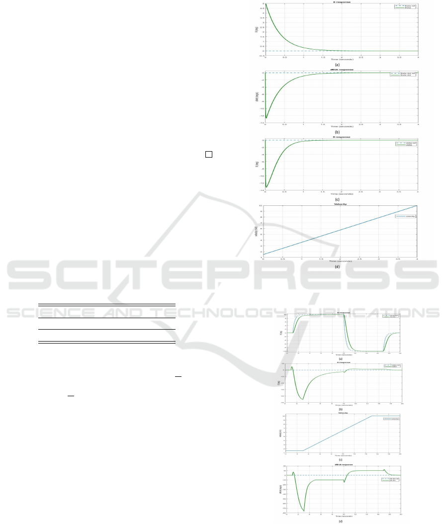
4 SIMULATION STUDIES
Although the proposed balancing controller is de-
signed based on the linearized model, for numerical
verifications, it is applied to the nonlinear model in
(6) to simulate the control performance. The system
parameters used are listed in Table 1.
Table 1: Parameters of the bicycle model used in the simu-
lations.
a 0.3957 m m 23.1 kg
b 1.053 m ` 0.4338 m
ε
0
20
◦
The controller design assumes that
(v
0
)
min
= 1.5m/s, (v
0
)
max
= 10m/s,

˙v
0
v
0

min
=
−2.5/s and

˙v
0
v
0

max
= 4/s. The four full-
state feedback gain matrices computed by
LMI’s are K
1
= [−185.12, −71.10,0.40],
K
2
= [−713.31,−273.49,22.39], K
3
=
[−693.76,−266.32,16.68], and K
4
=
[−801.19,−307.05,26.76]. In the first simula-
tion, we examine the stabilization properties of the
proposed controller under speed variations. It is de-
sired that the closed-loop system is stabilized around
the equilibrium point x = 0 which means that steering
the bicycle in a straight manner is of interests. The
initial state is set as x(0) =

5
◦
0
◦
/s 0
◦

T
.
Fig. 3 displays the responses of θ,
˙
θ, and δ of the
proposed controller as well as the speed history
used in the simulation . One can see that as the
bicycle accelerates linearly from 1.5m/s to 10m/s,
the controller is capable of centering the bicycle and
maintain the lateral stability. The maximum steering
angle is kept within 15
◦
. The second simulation is to
Figure 3: Simulated straight-line steering responses for the
proposed controller.
Figure 4: Simulated cornering responses for the proposed
controller.
examine the cornering performance of the proposed
controller. Cornering of the bicycle is achieved by
imposing a nonzero roll angle command θ
d
which
ICINCO 2019 - 16th International Conference on Informatics in Control, Automation and Robotics
38

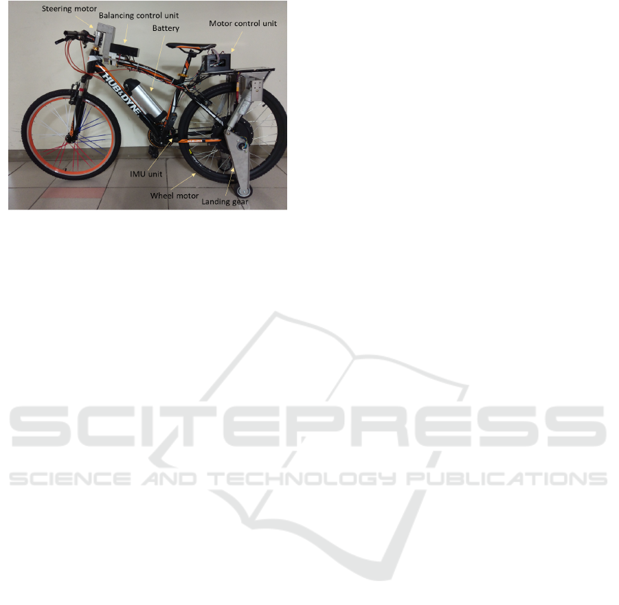
Figure 5: Photo of the prototype bicycle.
is generated as a filtered ±10
◦
square wave. The
simulated responses for the roll angle, steering angle,
velocity, and yaw rate are shown in Fig. 4. The
proposed controller is able to make the roll angle
track the desired command under speed variations.
The tracking of the roll angle command generates
corresponding steering angle response, which by (3)
and (8), causes the yaw rate response so that the bicy-
cle first turns right and then turns left. Notice that the
steering angle response exhibits undershoot during
cornering. Such a phenomenon, which matches the
experience of cornering an actual bicycle, is a typical
non-minimum-phase behavior due to the unstable
open-loop dynamics in (10).
5 EXPERIMENTAL
VERIFICATIONS
A prototype bicycle is constructed for experimental
validation. The bicycle contains a 500W brushless
DC wheel motor as the rear wheel. The motor speed
is regulated by a motor control unit which contains a
motor driver and an STM32F401RE MCU board. A
servo motor is installed on the pivot of the handlebar
to provide steering action. An inertial measurement
unit (IMU) which contains a three-axis accelerome-
ter and a three-axis gyro is attached to the bicycle
frame. The sensor fusion algorithm developed pre-
viously by the authors(Huang et al., 2018), which not
only considers the multi-axis coupling among the sen-
sor signals but also accounts for the dynamic effects
including the longitudinal acceleration and centrifu-
gal acceleration, is adopted to compute roll angle, roll
rate and yaw rate of the bicycle. Both the sensor
fusion and the control algorithm are implemented on
another STM32F401RE MCU board. To provide sup-
port at stationary position and low speeds, the bicycle
is also equipped with a set of landing gears which can
be actuated by linear electric actuators. The photo of
the prototype bicycle is shown in Fig. 5.
Experiments are conducted to compare the bal-
ancing performances of the proposed controller de-
signed as in the simulation section and a fixed-gain,
full-state feedback controller designed using LQR ap-
proach under constant speed assumption. First we
consider steering the bicycle in straight line. The re-
sponses in Fig. 6 indicate that the fixed-gain LQR
controller is unable to cope with speed changes that
the roll angle and steering angle start to diverge at
about 3s which eventually leads to bicycle fall. Fig.
7 shows the responses of the proposed controller. The
controller is able to maintain the lateral balance by
keeping the roll angle within 3
◦
. Notice that dur-
ing the experiment, the bicycle was supported by the
landing gears initially and at low speeds. Once the
speed reaches 0.5m/s, the land gears are lifted auto-
matically by the linear actuators and the bicycle is bal-
anced autonomously. The cornering performance of
the proposed controller is also examined experimen-
tally. A filtered square wave command for the roll an-
gle is adopted. According to the responses in Fig. 8,
the roll angle can basically follow the reference com-
mand.
6 CONCLUSIONS
This paper is devoted to the balancing control of a
self-driving bicycle . The proposed controller is a
convex combination of four linear, full-state feedback
controllers, which is specifically designed to cope
with the convex structure in the bicycle’s lateral dy-
namics under speed variations. The stability of the
control system is theoretically proved and a system-
atic procedure to compute the control gain matrices is
given. Both simulations and experiments verify that
the proposed controller can provide robust balancing
performance under various operating conditions. On-
going research efforts include incorporating cameras,
GPS sensors and so on to study collision avoidance
and autonomous navigation of the self-driving bicy-
cle.
ACKNOWLEDGMENT
The authors gratefully acknowledge the support pro-
vided by Ministry of Science and Technology in Tai-
wan.
Balancing Control of a Self-driving Bicycle
39

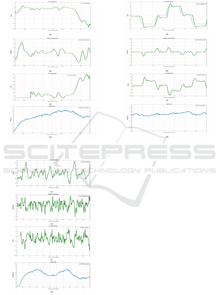
Figure 6: Experimental straight-line steering responses un-
der LQR control.
Figure 7: Experimental straight-line steering responses un-
der the proposed controller.
Figure 8: Experimental cornering responses under the pro-
posed controller.
REFERENCES
Astrom, K. J., Klein, R. E., and Lennartsson, A. (2005). Bi-
cycle dynamics and control: adapted bicycles for edu-
cation and research. IEEE Control Systems, 25(4):26–
47.
Beznos, A. V., Formal’sky, A. M., Gurfinkel, E. V., Jicharev,
D. N., Lensky, A. V., Savitsky, K. V., and Tch-
esalin, L. S. (1998). Control of autonomous motion
of two-wheel bicycle with gyroscopic stabilisation. In
Robotics and Automation, 1998. Proceedings. 1998
IEEE International Conference on, volume 3, pages
2670–2675 vol.3.
Cerone, V., Andreo, D., Larsson, M., and Regruto, D.
(2010). Stabilization of a riderless bicycle: A linear-
parameter-varying approach. In IEEE Control Syst.
Mag. Citeseer.
Huang, C.-F., Dai, B.-H., and Yeh, T.-J. (2018). De-
termination of motor torque for power-assist electric
bicycles using observer-based sensor fusion. Jour-
nal of Dynamic Systems, Measurement, and Control,
140(7):071019.
Huang, C. F., Tung, Y. C., and Yeh, T. J. (2017). Balanc-
ing control of a robot bicycle with uncertain center of
gravity. In 2017 IEEE International Conference on
Robotics and Automation (ICRA), pages 5858–5863.
Lowell, J. and McKel, H. D. (1982). The stability of bicy-
cles. American Journal of Physics, 50:1106–1112.
ICINCO 2019 - 16th International Conference on Informatics in Control, Automation and Robotics
40

Meijaard, J. P., Papadopoulos, J. M., Ruina, A., and
Schwab, A. L. (2007). Linearized dynamics equations
for the balance and steer of a bicycle: a benchmark
and review. In Proceedings of the Royal Society of
London A: Mathematical, Physical and Engineering
Sciences, volume 463, pages 1955–1982. The Royal
Society.
Sharp, R. S. (1971). The stability and control of motor-
cycles. Journal of mechanical engineering science,
13(5):316–329.
Slotine, J.-J. E. and Li, W. (1991). Applied nonlinear con-
trol, volume 199. Prentice hall Englewood Cliffs, NJ.
Tanaka, Y. and Murakami, T. (2004). Self sustaining bicycle
robot with steering controller. In Advanced Motion
Control, 2004. AMC ’04. The 8th IEEE International
Workshop on, pages 193–197.
Whipple, F. J. (1899). The stability of motion of a bicycle.
Quarterly Journal of Pure and Applied Mathematics,
30:312–348.
Zak, S. H. (2003). Systems and control, volume 174. Oxford
University Press New York.
Balancing Control of a Self-driving Bicycle
41