Lines to Planes Registration

Ales Jelinek and Adam Ligocki

Central European Institute of Technology, Purkynova 123, Brno, Czech Republic

Keywords:

Line, Plane, Registration, Least Squares, Optimization, Rigid Transformation, Data Fitting.

Abstract:

This paper deals with the Line-Plane registration problem. First we introduce the matter of geometrical object

ﬁtting and show the speciﬁcity of the Line-Plane combination. Then the method is derived to fulﬁl all usual

demands we put on a registration algorithm. Our algorithm works on any number of corresponding Line-Plane

pairs higher than three, providing more accurate results and better convergence, as this number gets higher.

Although the computation is non-linear by its nature, beneﬁts of the least squares optimization were preserved.

The algorithm is divided into a linear part dependant on the amount of input data and a non-linear part, which

is not, keeping efﬁciency in case of large data sets. All important features were experimentally tested and

proved to work.

1 INTRODUCTION

Registration of two sets of geometrical objects is a

longly solved problem in multiple disciplines of sci-

ence and engineering. Finding an optimal transfor-

mation, which brings one set as close to the other as

possible is an underlying principle connecting robotic

mapping (Cadena et al., 2016), object recognition

(Grimson and Lozano-P

erez, 1984), pose determina-

tion (Markley and Mortari, 2000) and other related

tasks. There is not a single type of transformation

to be discussed and neither a deﬁnition of ”close-

ness” is universal. Moreover, the geometrical objects

may vary in their nature (points, lines, planes, vec-

tors and rigid bodies to name the most common) and

there might not even be the same kind objects in both

sets. Another deﬁning difference is, whether we know

which objects from both sets correspond with each

other, or not.

All this diversity leads to a large number of ap-

proaches developed over the last decades (Cadena

et al., 2016), (Pomerleau et al., 2015), (Tam et al.,

2013). We are going to focus on rigid transformation

and known correspondences. There is plenty of algo-

rithms for registration problem with points in at least

one of the data sets (Wientapper and Kuijper, 2017),

(Olsson et al., 2006), (Ramalingam et al., 2010). The

Line-Line (Li et al., 2016) and Plane-Plane (Forstner

and Khoshelham, 2017) problem is addressed much

less, but we can still ﬁnd relevant literature. Surpris-

ingly, the Line-Plane problem draw minimal attention

over time and we were able to locate a single paper

(Chen, 1991) with working, yet somewhat unwieldy

algorithm.

In many practical situations, the lines are just ap-

proximations computed from point-like data, so the

Line-Plane task can be easily converted into a Point-

Plane equivalent. Though it is a viable option, stor-

ing point-like data might get very memory demanding

and sometimes these data do not exist at all. If extra

memory requirements are impractical, extra sampling

of lines to obtain points is terribly inefﬁcient. Lin-

ear and planar approximations can be used for further

processing (Cadena et al., 2016) while point-based

methods provide no additional value. Becoming inde-

pendent on points by direct solution of the Line-Plane

problem is therefore a useful addition to the state of

the art of the registration algorithms. This paper aims

to provide an alternative to (Chen, 1991) with more

favorable properties listed below:

• Our algorithm works on any number of corre-

sponding pairs N ≥ 3 in contrast to (Chen, 1991)

which needs exactly N = 3.

• The algorithm consists of two stages: I. Simple

linear computation with O(N) complexity (pro-

portional to the number of correspondences) and

II: Non-linear optimization independent on N.

• Addition and removal of a single correspondence

from the sets results in a constant time operation

on results precomputed in the ﬁrst stage.

• Initial guess to speed up the second stage can be

Jelinek, A. and Ligocki, A.

Lines to Planes Registration.

DOI: 10.5220/0007834906250632

In Proceedings of the 16th International Conference on Informatics in Control, Automation and Robotics (ICINCO 2019), pages 625-632

ISBN: 978-989-758-380-3

625

supplied.

• Provides metric directly describing quality of the

registration.

• Works for general planes and lines in 3D as well

as for general planes and lines lying in a single

plane (the case of line laser scanning mentioned

in (Chen, 1991), etc.).

To put the Line-Plane registration into the context

and provide ﬂuent introduction to actual derivation of

our method, we will discuss it together with a closely

related topic of methods designed for Vector-Vector

matching.

2 RELEVANT FACTS TO

LINE-PLANE REGISTRATION

As the work directly related our topic is so rare, we

will not start with traditional literature review, but

rather state the problem and than discuss its connec-

tions and differences from more established domains.

2.1 Problem Statement

Rigid transformation can be described by a rotation

matrix R and translation vector t

t acting on a vector in

the well known manner: x

= Rx

x + t

t. A line can be

described by a unit directional vector d

d and another

vector p

p representing a point lying on it. A general

plane is uniquely determined by a unit normal vector

n and the shortest distance l along this vector to the

origin. (Chen, 1991) formulates the problem as ﬁnd-

ing R and t

t satisfying the equations:

· Rd

= 0 (1)

and

· (Rp

t) = l

, (2)

for i = 1, 2, 3. As we are going to work with N ≥ 3

number of corresponding pairs, we will search for R

and t

t minimizing the error functions derived from (1)

and (2). For rotation R we get:

(R) =

∑

i=1

· Rd

)

, (3)

but generalization of (2) is not that straightforward.

(Chen, 1991) uses only three equations to ﬁnd R,

therefore the perfect match is guaranteed and the three

equalities (1) for i = 1,2,3 will be exactly valid.

When using N ≥ 3 equations, residual error depend-

ing on parametrization of the line will appear. p

an arbitrary point lying on the i-th line, so adding

some multiple of d

to p

should not inﬂuence any-

thing. Simple rearrangement of (2) gives:

·t

t = l

− n

· Rp

. (4)

Plugging p

+δd

instead of p

into (4) should not

inﬂuence the equality, but the following happens:

·t

t = l

− n

· Rp

− δn

· Rd

. (5)

The last term δn

· (Rd

) is guaranteed to be zero

if and only if N = 3, otherwise this is not necessar-

ily true and selection of p

could inﬂuence the result,

which is undesirable. To overcome this issue, we have

decided to use the point on the line closest to the ori-

gin of coordinates (p

= p

− (p

· d

) in place of

arbitrary p

, so the computation will get independent

of the choice of p

. Keeping the original notation we

arrive at the error function for translation:

(R,t

t) =

∑

i=1

· (R(p

− d

· p

)) +t

t) − l

)

. (6)

(Kamgar-Parsi and Kamgar-Parsi, 2011) advocate

even more robust approach to translation estimation,

pointing out dependency of the solution on selection

of the coordinate system. We found it much less sever

than the dependency on parametrisation of the lines,

so we have taken no precautions. In case of necessity,

our method should be modiﬁable in that manner at

cost of additional computational complexity.

Since evaluation of E

depends both on R and t

t and

there is a separate formula for R only, it is possible to

start with minimization of E

alone and than minimize

with given R. This way we follow order of the

operations during transformation and obtain sensible

results for both parameters, as presented in 2D case of

line segments in (Jelinek, 2018). Let us examine the

rotational part at ﬁrst.

2.2 Optimal Rotation

Lines and planes can be, among many other ways, de-

scribed using vectors. If only orientation is a con-

cern, than for lines, we extract the directional vectors

and for planes the normal vectors. In Line-Line and

Plane-Plane problems, the rotational part of registra-

tion boils down to alignment of two sets of vectors.

This operation is well described in literature and the

ﬁrst appearance was probably the Wahba’s problem

(Wahba, 1965) formulated as follows:

Given two sets of N points {v

, v

, ··· , v

} and

, v

, ··· , v

}, where N ≥ 2, ﬁnd the rotation matrix

R (i.e. the orthogonal matrix with determinant +1)

which brings the ﬁrst set into the best least squares

coincidence with the second. That is, ﬁnd R which

minimizes:

∑

i=1

k v

− Rv

. (7)

ICINCO 2019 - 16th International Conference on Informatics in Control, Automation and Robotics

626

2.2.1 A State of the Art Solution for Vectors

Therea are plenty of solutions, for example a decom-

position method by (Farrell et al., 1966), the Kab-

sch algorithm (Kabsch, 1976) and many other papers,

nicely surveyed in (Markley and Mortari, 2000). So-

lution using singular value decomposition (SVD) is

widely accepted and proceeds as follows.

Stationary vectors v

and rotated vectors v

are or-

ganized in matrices:

V =

























(8)

which provide the covariance matrix C:

C = V

, (9)

with

for transposition. SVD of the covariance ma-

trix expresses it as a product of three matrices:

C = USV

. (10)

The optimal rotation matrix is given by equation:

R = V





1 0 0

0 1 0

0 0 d





, (11)

where d = det(VU

). Note that the rotation R is an-

alytically expressed in terms of linear algebra provid-

ing a single optimal result. Although orthonormality

of the rotation matrix imposes non-linear constraints

on its nine elements, there is no need to reﬂect them

in the computation. SVD approach (8) - (11) repre-

sents state of the art solution, but it does not clearly

illustrate geometrical reason, why is that possible.

2.2.2 On Unnecessity of Non-linear Constraints

in Vector-Vector Registration

The example below brieﬂy shows, why for Vector-

Vector registration the constraints are naturally ful-

ﬁlled and why the Line-Plane case is more compli-

cated.

Let us again start with the two sets of unitary cor-

responding vectors (8). Coordinate frames of each

set are described by the orthonormal bases of three

vectors E = {e

, e

} and E

= {e

, e

}, both

equal to E

= {{1, 0, 0}, {0, 1, 0}, {0, 0,1}} at the be-

ginning. Then for every corresponding pair, we ﬁnd a

rotation R

which brings the registered vector v

into

coincidence with static v

. Axis of such rotation is

determined by the cross product v

× v

and the angle

corresponds to arccos(v

· v

). Frame E would than

Figure 1: All possible poses of the coordinate frame E

bringing vector v

(black) into perfect coincidence with v

(grey) from the second set. Red, green and blue circular

traces demarcate possible locations of the basis vectors of

correspond to R

as depicted in Fig. 1, where RGB

vectors are used to plot its axes.

But that is only one of inﬁnitely many possible

rotations. After the ﬁrst alignment, we can rotate E

about v

by an arbitrary angle and both vectors will

still perfectly coincide. Further rotation about v

re-

sults into a circular trace around v

for each e

(see

again Fig.1). One corresponding pair of vectors is

therefore not enough to specify orientation of the new

basis. On the other hand, we know exactly the magni-

tudes of projections of the basis vectors e

onto v

which remain constant for all possible poses of E.

With N ≥ 3, we can for every e

construct a system of

linear equations:

= V

, B







) · v







. (12)

For noise-less vecor sets V and V

, the least

squares solutions of the A

= B

systems yield the

coordinate frame E, which directly represents the ro-

tation R we sought for. Indeed, the approach sketched

above is inferior to the SVD solution, because it re-

quires N ≥ 3 even though it is proved that N ≥ 2 is

enough (Markley and Mortari, 2000), SVD works on

noised data as well and for large N its computational

costs are much lower. On the other hand, this example

clearly illustrates, why no non-linear constraints are

required in Vector-Vector registration. Distribution

of the invariant projections in matrices B

and (for

noised data) the properties of SVD encode enough in-

formation to retrieve proper rotation matrix R.

Lines to Planes Registration

627

2.2.3 The Line-Plane Problem Speciﬁcity

The geometric intuition behind the computation pro-

cedure described above can be easily extended to

Line-Plane registration. Using the notation from in-

troductory part of Section 2, the rotation which makes

a directional vector d

of a line orthogonal to a normal

vector n

of a plane, can be easily computed using

the products d

× n

and d

· n

, similar to the Vector-

Vector example above. After that operation, we can

freely rotate the coordinate frame not only about n

which corresponds to the previous example as well,

but also about the, now orthogonal, d

This is a deﬁning difference, because two degrees

of freedom in rotation cause loss of the constant size

projections, leaving us with no invariants to rely on.

Depiction in sense of Fig. 1 would show three over-

laying ring-like bands spanned around the n

vector.

It would be possible to use inequalities to describe

all possible locations of the basis vectors, but the ad-

vantage of implicitly present constraints embodied in

invariants would be lost anyway. This thought ex-

periment shows, inevitable non-linearity of the rota-

tional registration problem when lines and planes are

in question.

2.3 Optimal Translation

Contrary to the complicated matter of search for opti-

mal rotation, the translational part of the registration

turns out to be somewhat simpler. In case of formula

(2) by (Chen, 1991) it is a linear system of three equa-

tions with three variables. Due to our extension to

N ≥ 3 corresponding pairs we have to adopt the ad-

justment described in the problem statement in Sec-

tion 2.1. Then the optimal solution to minimization

of (6) turns out to be a straightforward least squares

computation as we will show near the end of the fol-

lowing section.

3 DERIVATION OF THE

METHOD

Previous discussion revealed, that our main concern

is minimization of (3) in search for optimal rotation

matrix R. We denote its elements as follows:

R =













(13)

and use them to write down the constraints, which ev-

ery proper rotation matrix has to fulﬁl:

· r

− 1 = 0,

· r

− 1 = 0,

· r

− 1 = 0,

· r

= 0,

· r

= 0,

· r

= 0

(14)

and then we deﬁne a vector r

r of R elements such that:

r =



··· r



. (15)

Next we take an outer product of n

and d









(16)

and organize it similar to r

r into a vector s



··· n



(17)

After this preparation, the error function (3) can

be expressed as:

(R) =

∑

i=1

· Rd

)

∑

i=1

· r

. (18)

Equation (18) in conjunction with constraints (14)

forms a starting point for further computation. In

principle, we try to ﬁnd a least squares solution best

fulﬁlling equality s

· r

r = 0 for i = 1 ···N, but non-

linear constraints prevent us from the straightforward

way of acquiring the result. Instead, we employ La-

grange multipliers λ

and formulate a Lagrange func-

tion:

r, λ

1,···,6

) =

∑

i=1

· r

−

∑

j=1

r), (19)

where c

r) are constraints (14). Partially differentiat-

ing this formula with respect to r

r yields the following

set of equations:

2λ

+ λ

= 2

∑

i=1

· r

2λ

+ λ

= 2

∑

i=1

· r

2λ

+ λ

= 2

∑

i=1

· r

2λ

+ λ

= 2

∑

i=1

· r

2λ

+ λ

= 2

∑

i=1

· r

2λ

+ λ

= 2

∑

i=1

· r

2λ

+ λ

= 2

∑

i=1

· r

2λ

+ λ

= 2

∑

i=1

· r

2λ

+ λ

= 2

∑

i=1

· r

(20)

ICINCO 2019 - 16th International Conference on Informatics in Control, Automation and Robotics

628

Differentiating of L

r, λ

1,···,6

) with respect to

1,···,6

gives back the constraints (14). (20) and (14)

form a system of non-linear equations to be solved

for r

r and λ

1,···,6

, directly leading to the rotation ma-

trix R. The crucial result is the independence of the

size of the non-linear system on the number of corre-

sponding pairs N. The information from an arbitrarily

high number of corresponding pairs is condensed in

the right side sums of (20). Detachment of search for

R from data aggregation allows better computational

optimization of both stages of the algorithm. Fur-

thermore, because every set of corresponding pairs is

fully speciﬁed by its sums, separate precomputation

allows constant time merging and splitting of sets, for

which the sums are known. This feature might be

utilized in correspondence search algorithms, making

our approach worth usage in this ﬁeld as well.

In many situations, an initial guess supplied to the

numerical solver is mandatory or beneﬁcial at least.

Any proper rotation matrix R

implies the values of

vector r

r, but we need a good guess of Lagrange mul-

tipliers λ

1,···,6

at the beginning as well. Fortunately,

proper R

automatically satisﬁes constraints (14) and

plugging its elements in place of r

r in the system of

equations (20) leaves us with linear system of nine

equations for six unknowns λ

1,···,6

. Common least

squares solution provides us with good initial setting

of λ

1,···,6

corresponding to R

The last step of the registration process is enumer-

ation of the optimal translation. In Section 2.1 we

have arrived at the error function (6):

(R,t

t) =

∑

i=1

· (R(p

− d

· p

)) + t

t) − l

)

With R being known, we can reformulate the prob-

lem into N equations:

·t

t = l

− n

· R(p

− d

· p

)), (21)

with variable t

t and the right side being known. An-

other overdetermined linear system suitable for least

squares solution have arisen in our computation.

Solving it yields the optimal translation we have been

looking for, while the sum of squared residuals pro-

vides accompanying error metric.

4 PRACTICAL VERIFICATION

Each theoretical result calls for empirical veriﬁca-

tion and comprehensive testing is mandatory for every

new method being deployed to practice. To test our

registration procedure, we have designed a few syn-

thetic tests exploring its main properties. The testing

code is written in Python 3.6.5 using NumPy 1.14.2

and SciPy 1.0.1 packages. We have not aimed for high

computational performance and the implementation is

not optimized in that respect. Underlying linear alge-

bra libraries and non-linear solvers are going to vary a

lot on different platforms in different applications, so

reasonably general benchmarking is highly problem-

atic. To provide at least some numbers, we can say

that on a 4.0A GHz CPU with lowly elaborated single

threaded implementation, the mean registration time

measured was a few milliseconds. Indeed, correspon-

dence count N and quality of initial guess inﬂuence

that number.

For error enumeration, there is a metric provided

by the method itself. For rotation, it is E

obtained

from equations (3) or (18) and for translation we use

(6), both available after every computation. We

refer it as an error function value. For the needs of

synthetic testing, we also employ Frobenius norm of

the difference between R estimated and the true rota-

tion matrix R

used during data generation. Denoting

this difference R

, the Frobenius error E

of the reg-

istration is:

(R) =

∑

j=1

∑

k=1

, (22)

where r

are elements of R

. This error metric is ob-

viously not available in real-life application, because

is unknown, but in synthetic testing it provides use-

ful comparison with the ground truth. Similar compu-

tation applies for translational part:

t) =

t −t

) · (t

t −t

), (23)

4.1 Stability and Convergence

The ﬁrst test is focused on reliability of convergence

to correct R, when imprecise initial guess is supplied

to the algorithm. If the guess is precise, the non-

linear solver terminates after the ﬁrst iteration leaving

the guess untouched, regardless the size of N. How-

ever if the guess does not comply with the data, the

solver might get caught in local minimum and pro-

vide suboptimal result. To test this behavior, we have

generated precisely corresponding pairs of line direc-

tions and plane normals and than rotated the direc-

tion with matrix R

. Next, the noise rotation matrix

was composed from arbitrary axis and angle be-

tween zero and a predeﬁned maximum. The initial

guess was than given by the product R

. Without

any noise in the data it is easy to detect suboptimal

results, because for correct registration, both E

and

are zero (up to certain negligible numerical error).

Success ratios for various N and initial guess error

amplitudes are organized in Tab. 1. One can clearly

Lines to Planes Registration

629

see importance of data set size for convergence of

the algorithm. For minimal input of three correspon-

dences, even a slight deviation of 3

◦

led to poten-

tial mismatches, however only two more Line-Plane

pairs moved this limit to 30

◦

, which is tremendous

improvement for its cost. Increasing N above a few

tens of pairs does not seem to help anything, when

convergence is in question.

Computation of optimal translation is a linear

problem featuring a single minimum for which an an-

alytical solution exists, so convergence is not an issue

in this case.

4.2 Noise Sensitivity and Accuracy

Second important experiment was performed to ex-

plore sensitivity of the method, when noise is present

in the input data. We have composed the noise matrix

using the same rules as in the previous experiment,

but now it was applied in conjunction with R

, when

the direction vectors were rotated. In this case, even

the optimal rotation produces some amount of error,

so neither error metric is zero any more.

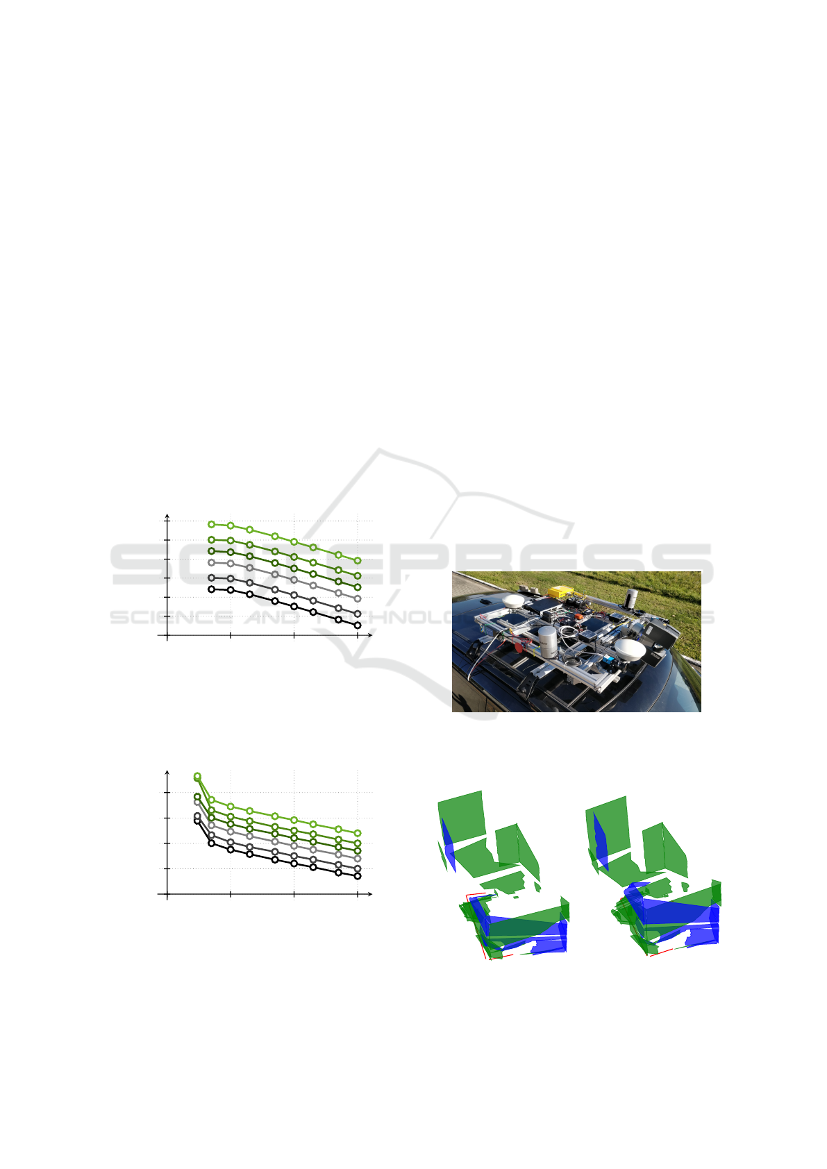
Figures 3 and 2 summarize the outcomes of this

experiment in case of rotation. For low N, espe-

cially for N = 3 and 5 we see an interesting behaviour.

(Chen, 1991) showed, that for non-degenerate set of

three Line-Plane pairs, there is an exact solution to the

registration problem, but we observe a non-zero error

. More than one reason is possible. First, in some

cases, the solution returned by the algorithm might

not be optimal (thus exhibiting non-zero error) in-

creasing the overall mean error from all experiments.

The second possible cause of these results is the num-

ber of vectors being involved. Three or ﬁve pairs

are simply not enough to provide a reliable statistics.

There is a good chance, that none of the vectors in-

volved was inﬂuenced by the noise with full ampli-

tude, resulting in more precise data than expected,

Table 1: Success ratio of correct convergence of the optimal

rotation search with given maximal error in initial guess of

the matrix and given number N of corresponding pairs used.

Error of the initial guess in degrees

1 3 5 10 30 50

3 1,00 0,99 0,98 0,97 0,89 0,77

5 1,00 1,00 1,00 1,00 0,99 0,91

10 1,00 1,00 1,00 1,00 1,00 0,99

30 1,00 1,00 1,00 1,00 1,00 1,00

50 1,00 1,00 1,00 1,00 1,00 1,00

100 1,00 1,00 1,00 1,00 1,00 1,00

300 1,00 1,00 1,00 1,00 1,00 1,00

500 1,00 1,00 1,00 1,00 1,00 1,00

1000 1,00 1,00 1,00 1,00 1,00 1,00

therefore lowering the mean error values. For higher

N, we see a gradual decrease of both error metrics,

proving an expectation, that larger data set should lead

to more precise outcomes. Comparison of E

and F

characteristics also proves feasibility of the E

error

metric. Although it tends to underestimate the error

for very small N, it corresponds to reliable F

based

on the original true rotation matrix.

The translational part of the registration was of

course tested as well. As its linear nature suggests,

we observe a gradual decrease in error for higher N,

(see Figures 5 and 4), but if N = 3, 5 there is more

to discuss. First, for cases when N = 3, there al-

ways exist an exact solution to the system of equa-

tions (21), making the expected error E

zero (not

plotted in Fig. 4). Nevertheless, the Frobenius error

(Fig. 5) derived from true translation shows non-

proportionally high values for N = 3. This behavior

is even stronger argument against Line-Plane registra-

tion with only three samples, than similar effect man-

ifesting in rotation enumeration. The N = 5 case is

still inﬂuenced by error underestimation, but at least,

we get reasonable values to alarm our attention. For

higher N, E

nicely reﬂects true error behavior de-

Number of points N

−8

−7

−6

−5

−4

−3

−2

Figure 2: Error function (3) divided by N

reﬂecting ex-

pected deviation from true rotation matrix for various num-

ber of points N. Paths in the chart belong to 1

◦

, 2

◦

, 5

◦

, 10

◦

peak error in line directions in bottom up order.

Number of points N

−4

−3

−2

−1

Figure 3: Frobenius error reﬂecting real deviation from true

rotation matrix for various number of points N. Paths in

the chart belong to 1

◦

, 2

◦

, 5

◦

, 10

◦

, 20

◦

peak error in line

directions in bottom up order.

ICINCO 2019 - 16th International Conference on Informatics in Control, Automation and Robotics

630

scribed by F

and can be safely used to determine ex-

pected error of the computation.

4.3 Real Data Testing

Truly empirical experiments turned out to be some-

what problematic to perform, because acquiring

highly accurate control measurements is quite hard.

Our real-life application is calibration of surround

sensing devices for mobile robots (Zalud et al., 2015),

(Kocmanova et al., 2013), in this case a mutual pose

of 3D and 2D sensing laser scanners (see Fig. 6). Each

of these devices has its own frame of coordinates, but

its origin is inside of the body of the device, so tak-

ing exact measurements is extremely difﬁcult. Veriﬁ-

cation therefore does not come from direct measure-

ment, but rather from comparison of overlay of the

point clouds measured by the devices, before and after

the calibration transformation is applied. This overlay

can be enumerated by multitude methods resulting in

many numerical values (Pomerleau et al., 2015), but

the essence of all comparisons is simple: The point

Number of points N

−6

−5

−4

−3

−2

−1

Figure 4: Error function (6) divided by N

reﬂecting ex-

pected deviation from true translation vector for various

number of points N. Paths in the chart belong to 1, 2, 5,

10, 20 and 50 percent peak error with respect to maximal

mutual distance of lines and planes (in bottom up order).

Number of points N

−3

−2

−1

Figure 5: Frobenius error reﬂecting real deviation from true

translation vector for various number of points N. Paths in

the chart belong to 1, 2, 5, 10, 20 and 50 percent peak error

with respect to maximal mutual distance of lines and planes

(in bottom up order).

clouds after calibration ﬁt together much better than

without it (see Fig. 7), despite the metric used. How-

ever humble this number-less experiment looks on the

paper, it is a clear evidence of functionality of the reg-

istration method described above.

5 CONCLUSIONS

The Line-Plane registration problem is surprisingly

unexplored in the literature. This paper provides in-

tuitive introduction into peculiar details of the topic

and, to our best knowledge, presents a solution with

properties exceeding any other method approaching

this problem.

Our algorithm works with any number N of the

corresponding Line-Plane pairs greater than three a

splits the computation into O(N) complex linear part

and N-independent non-linear part. The error metric

is supplied, which allows reliability evaluation of the

computation and the method also works, if all lines

lie in a single plane. Increasing size N of the dataset

leads to higher stability of the computation as well

as higher precision of the results. If an initial guess

of the transformation is provided, the computation is

faster and more robust. All these results were practi-

Figure 6: The Atlas sensory platform designed for surround

sensing of autonomous vehicles. Line-Plane registration is

used for mutual pose calibration of the FARO laser scanner

and both Velodyne laser scanners.

(a) Rough pose estimate. (b) After registration.

Figure 7: Line-Plane registration in a calibration scenario.

Lines to Planes Registration

631

cally veriﬁed in Section 4. Based on the experiments,

we strongly advocate to use at least N = 5 for better

robustness, which contradicts many methods requir-

ing N = 3.

ACKNOWLEDGEMENTS

The research was supported by ECSEL JU under the

project H2020 737469 AutoDrive - Advancing fail-

aware, fail-safe, and fail-operational electronic com-

ponents, systems, and architectures for fully auto-

mated driving to make future mobility safer, afford-

able, and end-user acceptable. This research has been

ﬁnancially supported by the Ministry of Education,

Youth and Sports of the Czech republic under the

project CEITEC 2020 (LQ1601).

REFERENCES

Cadena, C., Carlone, L., Carrillo, H., Latif, Y., Scaramuzza,

D., Neira, J., Reid, I., and Leonard, J. J. (2016). Past,

Present, and Future of Simultaneous Localization and

Mapping: Toward the Robust-Perception Age. IEEE

Transactions on Robotics, 32(6):1309–1332.

Chen, H. (1991). Pose determination from line-to-plane

correspondences: existence condition and closed-

form solutions. IEEE Transactions on Pattern Analy-

sis and Machine Intelligence, 13(6):530–541.

Farrell, J. L., Stuelpnagel, J. C., Wessner, R. H., Velman,

J. R., and Brook, J. E. (1966). A Least Squares Esti-

mate of Satellite Attitude (Grace Wahba). SIAM Re-

view, 8(3):384–386.

Forstner, W. and Khoshelham, K. (2017). Efﬁcient and

Accurate Registration of Point Clouds with Plane to

Plane Correspondences. In 2017 IEEE International

Conference on Computer Vision Workshops (ICCVW),

pages 2165–2173. IEEE.

Grimson, W. E. L. and Lozano-P

erez, T. (1984). Model-

Based Recognition and Localization from Sparse

Range or Tactile Data. The International Journal of

Robotics Research, 3(3):3–35.

Jelinek, A. (2018). On registration of vector maps with

known correspondences. In 2018 ELEKTRO, pages

1–6. IEEE.

Kabsch, W. (1976). A solution for the best rotation to relate

two sets of vectors. Acta Crystallographica Section A,

32(5):922–923.

Kamgar-Parsi, B. and Kamgar-Parsi, B. (2011). Matching

2D image lines to 3D models: Two improvements and

a new algorithm. In CVPR 2011, pages 2425–2432.

IEEE.

Kocmanova, P., Zalud, L., and Chromy, A. (2013). 3D prox-

imity laser scanner calibration. In 2013 18th Interna-

tional Conference on Methods & Models in Automa-

tion & Robotics (MMAR), pages 742–747. IEEE.

Li, X., Zhang, Y., Shang, Y., and Liu, H. (2016). Proba-

bilistic approach for maximum likelihood estimation

of pose using lines. IET Computer Vision, 10(6):475–

482.

Markley, F. L. and Mortari, D. (2000). How to estimate

attitude from vector observations. Advances in the As-

tronautical Sciences, 103(PART III):1979–1996.

Olsson, C., Kahl, F., and Oskarsson, M. (2006). The Reg-

istration Problem Revisited: Optimal Solutions From

Points, Lines and Planes. In 2006 IEEE Computer

Society Conference on Computer Vision and Pattern

Recognition - Volume 1 (CVPR’06), volume 1, pages

1206–1213. IEEE.

Pomerleau, F., Colas, F., and Siegwart, R. (2015). A Re-

view of Point Cloud Registration Algorithms for Mo-

bile Robotics. Foundations and Trends in Robotics,

4(1):1–104.

Ramalingam, S., Taguchi, Y., Marks, T. K., and Tuzel,

O. (2010). P2Pi: A Minimal Solution for Reg-

istration of 3D Points to 3D Planes BT - Com-

puter Vision–ECCV . . . . Computer Vision–ECCV . . . ,

6315(Chapter 32):436–449.

Tam, G. K. L., Zhi-Quan Cheng, Yu-Kun Lai, Langbein,

F. C., Yonghuai Liu, Marshall, D., Martin, R. R.,

Xian-Fang Sun, and Rosin, P. L. (2013). Registration

of 3D Point Clouds and Meshes: A Survey from Rigid

to Nonrigid. IEEE Transactions on Visualization and

Computer Graphics, 19(7):1199–1217.

Wahba, G. (1965). A Least Squares Estimate of Satellite

Attitude. SIAM Review, 7(3):409–409.

Wientapper, F. and Kuijper, A. (2017). Unifying Alge-

braic Solvers for Scaled Euclidean Registration from

Point, Line and Plane Constraints. In Lecture Notes

in Computer Science, pages 52–66. Springer Interna-

tional Publishing.

Zalud, L., Kocmanova, P., Burian, F., Jilek, T., Kalvoda, P.,

and Kopecny, L. (2015). Calibration and Evaluation

of Parameters in A 3D Proximity Rotating Scanner.

Elektronika ir Elektrotechnika, 21(1):3–12.

ICINCO 2019 - 16th International Conference on Informatics in Control, Automation and Robotics

632