Parallel Streaming Implementation of Online Time Series Correlation

Discovery on Sliding Windows with Regression Capabilities

Boyan Kolev

, Reza Akbarinia

, Ricardo Jimenez-Peris

, Oleksandra Levchenko

Florent Masseglia

, Marta Patino

and Patrick Valduriez

Inria and LIRMM, Montpellier, France

LeanXcale, Madrid, Spain

Universidad Politecnica de Madrid (UPM), Madrid, Spain

Keywords: Time Series Correlation and Regression, Data Stream Processing, Distributed Computing.

Abstract: This paper addresses the problem of continuously finding highly correlated pairs of time series over the most

recent time window and possibly use the discovered correlations to select features for training a regression

model for prediction. The implementation builds upon the ParCorr parallel method for online correlation

discovery and is designed to run continuously on top of the UPM-CEP data streaming engine through efficient

streaming operators.

1 INTRODUCTION

Consider a big number of streams of time series data

(e.g. stock trading quotes), where we need to find

highly correlated pairs for the latest window of time

(say, one hour), and then continuously slide this

window to repeat the same search (say, every

minute). Doing this efficiently and in parallel could

help gather important insights from the data in real

time (Figure 1). This has been recently addressed by

the ParCorr parallel incremental sketching approach

(Yagoubi et al., 2018), which scales to 100s of

millions of parallel time series, and achieves 95%

recall and 100% precision. An interesting aspect of

the method is the discovery of time series that are

highly correlated to a certain subset of the time series,

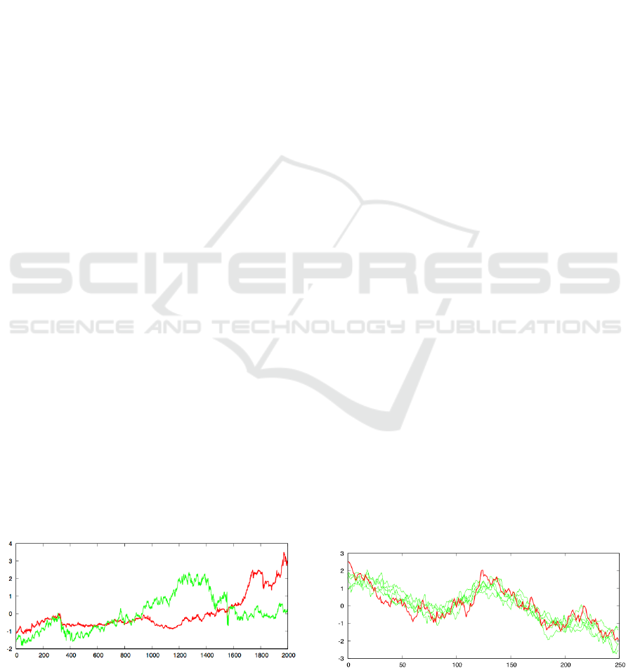
which we call targets (Figure 2). This concept has

many applications in different domains (finance,

Figure 1: Example of a pair of time series that the method

found to be highly correlated over the first several sliding

windows of 500 time points, but not thereafter.

retail, etc.), where we would like to use the correlates

of a target as predictors to forecast the value of the

target for the next time window.

Such challenges have been identified by use case

scenarios, defined in the scope of the

CloudDBAppliance project (CDBA, 2019), which

aims to provide a database-as-a-service appliance

integrating several data management technologies,

designed to scale vertically on many-core

architectures. These include an operational database,

an analytical database, a data lake, and a data

streaming engine. To face these requirements, the

ParCorr method was implemented as a continuous

query for the highly scalable streaming engine and

enhanced with regression capabilities to provide for

per-window prediction of target values. In this paper,

we present the details of this implementation,

following a brief overview of the streaming engine

and the ParCorr method.

Figure 2: Example of a target time series (red) and its top

correlates (green) discovered by the method.

Kolev, B., Akbarinia, R., Jimenez-Peris, R., Levchenko, O., Masseglia, F., Patino, M. and Valduriez, P.

Parallel Streaming Implementation of Online Time Series Correlation Discovery on Sliding Windows with Regression Capabilities.

DOI: 10.5220/0007843806810687

In Proceedings of the 9th International Conference on Cloud Computing and Services Science (CLOSER 2019), pages 681-687

ISBN: 978-989-758-365-0

 2019 by SCITEPRESS – Science and Technology Publications, Lda. All r ights reserved

681

2 STREAMING ENGINE

OVERVIEW

Stream Processing (SP) is a novel paradigm for

analyzing in real-time data captured from

heterogeneous data sources. Instead of storing the

data and then processing it, the data is processed on

the fly, as soon as it is received, or at most a window

of data is stored in memory. SP queries are

continuous queries run on a (infinite) stream of

events. Continuous queries are modeled as graphs

where nodes are SP operators and arrows are streams

of events. SP operators are computational boxes that

process events received over the incoming stream and

produce output events on the outgoing streams. SP

operators can be either stateless (such as projection,

filter) or stateful, depending on whether they operate

on the current event (tuple) or on a set of events (time

window or number of events window). Several

implementations went out to the consumer market

from both academy and industry, such as Borealis

(Ahmad et al., 2005), Infosphere (Pu et al., 2001),

Storm

, Flink

and StreamCloud (Gulisano et al.,

2012). Storm and Flink followed a similar approach

to the one of StreamCloud in which a continuous

query runs in a distributed and parallel way over

several machines, which in turn increases the system

throughput in terms of number of tuples processed per

second. The streaming engine UPM-CEP (Complex

Event Processing) adds efficiency to this parallel-

distributed processing being able to reach higher

throughput using less resources. It improves the

network management, reduces the inefficiency of the

garbage collection by implementing techniques such

as object reutilization and takes advantage of the

novel Non Uniform Memory Access (NUMA)

multicore architectures by minimizing the time spent

in context switching of SP threads/processes.

The UPM-CEP JCEPC (Java CEP Connectivity)

driver hides from the applications the complexity of

the underlying cluster. Applications can create and

deploy continuous queries using the JCEPC driver as

well as register to the source streams and subscribe to

output streams of these queries. During the

deployment the JCEPC driver takes care of splitting a

query into sub-queries and deploys them in the CEP

cluster. Some of those sub-queries can be

parallelized.

http://storm.apache.org/

3 METHOD OVERVIEW

The ParCorr time series correlation discovery

algorithm (Yagoubi et al., 2018) is based on a work

on fast window correlations over time series of

numerical data (Cole et al., 2005), and concentrates

on adapting the approach for the context of a big

number of parallel data streams. The analysis is done

on sliding windows of time series data, so that recent

correlations are being continuously discovered in

nearly real-time. At each move of the sliding window,

the latest elements of the time series are taken as

multi-dimensional vectors. As a similarity measure

between such vectors, we take the Euclidean distance,

since it is related to the Pearson correlation

coefficient if applied to normalized vectors. Since the

sliding window can result in a very high number of

dimensions of time series vectors, which makes them

very expensive to be compared to each other, a major

challenge the algorithm addresses is the reduction of

the dimensionality in a way that nearly preserves the

Euclidean distances. For this purpose, random

projection approach is adopted, where each high-

dimensional vector is transformed into a low-

dimensional one (called “sketch” of the vector), by

applying a product with a specific transformation

matrix, the elements of which are randomly selected

from the values of either -1 or 1. This approach

guarantees with high probability that the distance

between any pair of original vectors correspond to the

distance between their sketches. Furthermore, to

simplify the comparing across sketches, each sketch

vector is partitioned into subvectors (e.g. two-

dimensional), so that for example a 30-dimensional

sketch vector is broken into 15 two-dimensional

subvectors. Then, discrete grid structures (in the

example, 15 two-dimensional grids) are built and

subvectors are assigned to grid cells, so that close

subvectors are grouped in the same grid cells. This

process essentially performs a locality-sensitive

hashing of high-dimensional time series vectors,

where close vectors are discovered by searching for

pairs of vectors, which are represented together in a

high number of grid cells. Since this can output false

positives, the candidate pairs are explicitly verified by

computing the actual distance between them.

This outlines four main steps of the algorithm:

 Sketching: computation and partitioning of

sketches;

 Collocation: grouping together all time series

assigned to the same grid cell;

 Correlation: finding frequently collocated pairs as

https://flink.apache.org/

ADITCA 2019 - Special Session on Appliances for Data-Intensive and Time Critical Applications

682

Figure 3: The four main steps of the time series correlation discovery algorithm, implemented as parallel stateful streaming

operators, with intermediate shuffles of data.

candidates for correlation;

 Verification: computing the actual correlation of

each candidate pair to filter out false positives.

To provide prediction capabilities, an additional step

trains a regression model that takes into account the

correlates of time series that are considered of interest

for prediction and called “targets”. Only correlated

pairs that involve at least one target time series are

considered for discovery. All correlates of a target are

considered as predictors and passed to a linear

regression model, which approximates the target as a

linear function of its correlates.

4 IMPLEMENTATION

The implementation involves four stateful streaming

operators (Figure 3), each processing incoming tuples

in the context of the current window, taking into

account the current state of the window. Thanks to the

flexible API of the streaming engine that provides

low level primitives for implementing custom

operators, each operator can process incoming tuples

on-the-fly and hence emit resulting tuples as early as

possible. This guarantees a real pipelined flow of data

that allows for outputting early results.

4.1 Data Input and Output

All tuples processed by the streaming engine must

contain associated timestamps. The schemas of the

input stream and the two output streams are as

follows:

 Input stream

o timestamp timestamp

o tsId string

o value float

 Basic output stream

o timestamp timestamp

o tsId1 string

o tsId2 string

o correlation float

 Extended output stream

o timestamp timestamp

o target string

o predictors string[]

o coefs float[]

For input data tuples, timestamp identifies the point

in time, for which the value of a particular time

series (tsId) is taken. Examples can be product price

at a given moment, volume of sales for a given time

unit (say 1 minute), etc. For the method to work

correctly, each time series must have value at each

timestamp. If such is not provided, the sketching

operator will assume repetition of the last value.

Normally, time units should be aligned to data update

frequencies.

Basic output tuples show pairs of identifiers of the

time series (tsId1 and tsId2), which were found to

be highly correlated at the window, represented by the

provided timestamp, together with the Pearson

correlation coefficient.

For the regression extensions, each of the

extended output tuples shows the approximation of a

specific target, as a list of its predictors and the

corresponding coeficients for each predictor in

the linear model. Thus, the next value of target can

be predicted as function of predictors, using the

formula:

  











 







(1)

where n is the number of predictors, P

is the next

value of the time series whose identifier is stored in

predictors[i-1], C

is the regression coefficient

of P

stored in coefs[i], and C

is the intercept of

the linear regression model stored in coefs[0].

The arrays predictors and coefs are actually

output as pipe-separated list of values. For example,

the following output tuple:

target: "Demand",

predictors: "Price|Discount|Precip",

Parallel Streaming Implementation of Online Time Series Correlation Discovery on Sliding Windows with Regression Capabilities

683

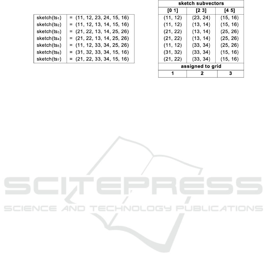
(a) a sample of time series sketches (b) sketch partitioning

Figure 4: The sketching operator computes sketches at each sliding window and assigns time series (identifiers) to grid cells.

coefs: "1.3|3.9|2.5|-0.7"

says that the next value of demand can be

approximated once the values of price, discount, and

precip are known, with the following expression:

Demand ~= 1.3 + 3.9*Price

+ 2.5*Discount - 0.7*Precip

4.2 Model Parameters

The model can be configured by a number of

parameters, which can be roughly divided in two

groups: functional parameters and method

parameters.

Functional parameters are determined by the

application requirements. Sliding windows are

defined in terms of size of the window (windowSize)

and size of a basic window (windowSlide, the step

at which a sliding window advances). For example, if

we consider a time unit of one minute, a basic window

of size 5 and a window of size 60, this means that

method execution will be triggered every 5 minutes

and will run on time series data for the last 60

minutes. Other functional parameters are the desired

correlation threshold minCorr (e.g., the application

needs all pairs with Pearson correlation above 0.9)

and the searchInverse flag that indicates whether

highly negative correlations (e.g., less than -0.9) are

to be also discovered. The optional targets

parameter is a regular expression that specifies the

identifiers of target time series; the simplest form is a

pipe-separated list of time series identifiers that will

be considered as targets.

Method parameters can control the tradeoff

between efficiency (the time to response at each

window slide) and accuracy (what percentage of all

highly correlated pairs will be discovered). That is

mostly determined by the grid cell size and the

candidate threshold, i.e. the minimum number of

grids, in which two time series should be collocated

in order to be considered as candidates for correlation.

Larger grid cells (i.e. more time series assigned to the

same cell) and lower candidate threshold lead to

higher number of candidate pairs to process (slower

execution), but lower probability to miss a true

positive (higher accuracy). Another important

parameter is the sketch size, which determines the

reduced dimensionality and can also control the same

tradeoff (lower dimensional sketch vectors lead to

faster execution, but also to lower probability of

preserving the distances). If linearSearch is set to

true, an exhaustive search through all possible pairs

will be done, instead of running the sketching

method, hence all other method parameters will be

ignored. Linear search is also parallelized, but much

slower, as it naively explores the full search space.

However, it guarantees to discover 100% of the

correlations, so might be the preferred method for

applications with a smaller number of time series that

need exact responses. This parameter has also been

used for comparing and evaluating the performance

benefits of the sketching method and its accuracy

tradeoff.

The model parameters are summarized below:

 Functional parameters:

o windowSize integer

o windowSlide integer

o minCorr float

o searchInverse boolean

o targets string

 Method parameters:

o sketchSize integer

o cellSize float

o threshold integer

o linearSearch boolean

4.3 Streaming Operators

Figure 3 depicts the algorithm workflow across the

ADITCA 2019 - Special Session on Appliances for Data-Intensive and Time Critical Applications

684

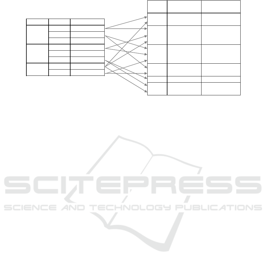
(a) each grid cell contains the ids of

collocated time series

(b) candidate clusters are explored for

frequently collocated time series ids

Figure 5: The collocation and correlation operators explore grid cells to identify candidate pairs.

streaming operators. The parallelization of the

algorithm is quite straightforward – sketches of time

series vectors on parallel data streams are computed

in parallel, which is followed by an additional shuffle

step that groups together the identifiers of time series

that fit in the same grid cell; then groups are explored

for discovering frequent pairs. Since the streaming

engine operates in a distributed environment,

operators have multiple instances, handling different

partitions of data in parallel. This requires shuffles of

intermediate data across operator instances and the

partitioning is based on a key from the schema of the

intermediate dataset. In figures, we use the

Key=>Value notation to show which fields are used

as partition keys.

4.3.1 Sketching

The first operator consumes the incoming data,

represented as a stream of (timestamp, tsId, value)

tuples. Its incoming data partitioning ensures that all

values of the same time series id (tsId) are routed to

the same operator instance.

First, the operator identifies sliding windows and

at each window computes the sketch of each time

series. This computation is done incrementally, i.e. at

each slide of the window, the sketches are simply

incrementally updated (instead of recomputed),

taking into account only the difference compared to

the previous position of the sliding window. Since the

method requires that sketches be computed on

normalized vectors, means and standard deviations

are computed (also incrementally) for each sliding

window. Then, they are applied directly in the

formula for computing the sketches, which results in

sketch values as if computed on a normalized

window.

As a running example, let us consider seven time

series with sketches as shown on Figure 4a. Each

sketch vector is partitioned into three pairs

(subvectors). The i

pair of the sketch vector for each

time series s goes to a grid i. The values of the i

pair

determine where in that grid the identifier s is placed.

Thus, each time series id is associated to exactly 3

grid cells – one at each grid (Figure 4b). Each cell is

identified by cellId, composed by the grid index and

the two dimensions of the grid cell. After this

processing, the sketching operator emits these

associations as (cellId, tsId) pair tuples.

4.3.2 Collocation

The second operator uses cellId as key and groups in

partitions all time series identifiers that belong to the

same cell (Figure 5a). Then, for each identifier in a

partition, the operator emits a key-value pair that

maps the time series identifier to its relevant part of

the partition (Figure 5b). The relevant part of a

partition with respect to a time series t consists of t

itself and the time series with identifiers higher than

t. We call that a “candidate cluster of time series”.

Clusters with just one element are ignored, because

pairs cannot be derived out of them. If the targets

parameter is specified, a filter is applied so that only

those key-value tuples that correspond to targets be

emitted at this step.

4.3.3 Correlation

The third operator uses tsId as key and for each time

TS ID TS clusters candidate pairs

(f ≥ 2/3)

, ts

grid cell TS IDs

(11, 12)

, ts

(21, 22)

, ts

(31, 32)

(13, 14)

, ts

(23, 24)

(33, 34)

, ts

(15, 16)

, ts

(25, 26)

, ts

Parallel Streaming Implementation of Online Time Series Correlation Discovery on Sliding Windows with Regression Capabilities

685

Figure 6: The architecture of the streaming operators, with all intermediate streams. The correlation and verification operators

keep copies of the current window of raw time series data, needed for computing the actual correlations.

series identifier t explores its associated candidate

clusters to find those time series ids that are

frequently collocated with t. In the example on Figure

5b, three pairs satisfy the given candidate threshold f

(i.e. they are seen together in the same cell in 2 out of

3 grids) and are hence considered as candidates for

correlation.

To facilitate the next step, the Correlation operator

keeps a copy of the current window of time series raw

data (Figure 6), partitioned by identifier. This assures

that every candidate pair (ts

, ts

) will be collocated

with the raw time series (data

) of ts

at the same

operator instance, since the candidate pair is keyed by

. Thus, each instance of the Correlation operator

performs a join between its candidate pairs and the

local partition of the raw time series table and emits

the triplet (ts

, ts

, data

4.3.4 Verification

Each candidate (ts

, ts

) emitted by the Correlation

operator must be now explicitly verified by

computing the actual Pearson correlation between the

two time series to check whether it satisfies the

desired correlation threshold. This requires another

lookup into the original time series window, in order

to get the raw time series (data

), this time of ts

. For

this reason, the Verification operator also keeps a

copy of the current window of time series raw data,

this time having ts

as key (Figure 6). Finally, the

correlation of (data

, data

) is computed and, if higher

than the threshold, the candidate is emitted to the

correlations output.

4.3.5 Regression

The Verification operator makes sure that the data

processed by it is already partitioned by target time

series id, i.e. all the predictors of a particular target,

together with their data for the last window, are

collocated at the same instance with the target. This

http://commons.apache.org/proper/commons-math/

userguide/stat.html

avoids additional shuffles of intermediate data and

makes it easy for Regression to train a linear

regression model for each of the target time series,

consuming immediately the output of the Verification

operator. So, Regression is stateless and is simply

implemented as a class that operates within the

Verification operator (R box of Figure 6). The

implementation uses the Statistics package of the

Apache Commons Math library

5 CONCLUSIONS

We presented a parallel streaming implementation of

the ParCorr method for window correlation discovery

on time series data, enhanced with regression

capabilities, in the context of the CloudDBAppliance

project. The implementation leverages the

development of custom streaming operators that

boosts the performance and minimizes the response

time by optimizing intra-operator communication and

utilizing pipelining of intermediate data. As a subject

to further work, we will study experimentally the

performance benefits of this implementation,

compared to other streaming architectures, with

respect to latency of the first results and response time

of the entire output at each time window.

ACKNOWLEDGEMENTS

This work has been partially funded by the European

Union's Horizon 2020 Programme, project

CloudDBAppliance, grant 732051.

REFERENCES

Ahmad, Y., Berg, B., Cetintemel, U., Humphrey, M.,

Hwang, J., Jhingran, A., Maskey, A., Papaemmanouil,

ADITCA 2019 - Special Session on Appliances for Data-Intensive and Time Critical Applications

686

O., Rasin, A., Tatbul, N., Xing, W., Xing, Y., Zdonik,

S., 2005, Distributed Operation in the Borealis Stream

Processing Engine. ACM SIGMOD International

Conference on Management of Data (2005), pp 882–

884.

CDBA, 2019. The CloudDBAppliance Project. http://

clouddb.eu

Cole, R., Shasha, D., Zhao, X., 2005. Fast Window

Correlations over Uncooperative Time Series. In:

Proceedings of the International Conference on

Knowledge Discovery and Data Mining (SIGKDD).

ACM, pp 743–749.

Gulisano, V., Jimenez-Peris, R., Patino-Martinez, M, C.

Soriente, C., Valduriez, P., 2012. Streamcloud: An

Elastic and Scalable Data Streaming System. IEEE

Trans. Parallel Distrib. Syst. 23(12), pp 2351–2365.

Pu, C., Schwan, K., Walpole, J., 2001. Infosphere Project:

System Support for Information Flow Applications.

SIGMOD Record 30(1) (2001), pp 25–34.

Yagoubi, D.-E., Akbarinia, R., Kolev, B., Levchenko, O.,

Masseglia, F., Valduriez, P., Shasha, D., 2018. ParCorr:

Efficient Parallel Methods to Identify Similar Time

Series Pairs across Sliding Windows. Data Mining and

Knowledge Discovery, vol. 32(5), pp 1481-1507.

Springer.

Parallel Streaming Implementation of Online Time Series Correlation Discovery on Sliding Windows with Regression Capabilities

687