Data Mining using Morlet Wavelets for Financial Time Series

Reginald Bolman and Thomas Boucher

Department of Mathematics, Texas A&M University-Commerce, 2200 Campbell St, Commerce TX, U.S.A.

Keywords:

Morlet Wavelets, Financial Time Series Datasets, Datamining, Financial Time Series Analysis, Wavelet

Analysis, Time Series Power Comparison.

Abstract:

Wavelets are a family of signal processing techniques which have a growing popularity in the artiﬁcial in-

telligence community. In particular, Morlet wavelets have been applied to neural network time series trend

prediction, forecasting the effects of monetary policy, etc. In this paper, we discuss the application of Morlet

wavelets to discover the morphology of a time series cyclical components and the unsupervised data mining

of ﬁnancial time series in order to discover hidden motifs within the data. To perform the analysis of a given

time series and form a comparison between the morphologies this paper proposes the implementation of the

“Bolman Time Series Power Comparison” algorithm which will extract the pertinent time series motifs from

the underlying dataset.

1 INTRODUCTION

Wavelet methods have seen popular application to

many different ﬁelds in computer science, engineer-

ing and mathematics to solve a wide range of prob-

lems. Most recently, wavelets have seen their applica-

tion to econometric time series forecasting, analyzing

the effects of monetary policy and modeling econo-

metric dynamics due in part to their ability to decom-

pose a signal into its respective time series compo-

nents. Considering how economics exhibit chaotic

dynamics and are complex systems with potentially

tens or hundreds of interacting variables at differing

time scales, wavelet methods have therefore become

an invaluable analysis tool for ﬁnancial time series in-

vestigations.

In the realm of individual investors and institu-

tional trading the “rule of 4” is common in the indus-

try; a trade entry/exit strategy based on position time

frames which are a multiple of 4. A trader might plan

trades on a daily horizon and since there are 8 hours in

a trading day the trader would position himself based

on a 2 hour time interval and judge entry/exit signals

based on 60 minute intervals. Hence, planning hori-

zons are an integral component to trading market se-

curities and the success of such a trading strategy is

in many instances dependent on the optimization of

these trading intervals. Therefore, It’s not surprising

that ﬁnancial time series in aggregate across millions

of traders exhibit wildly different behavior based on

which time frame is being analyzed.

Wavelets are a multi-resolution decomposition

technique and when applied to econometric data, pro-

vide insight into variables who’s relationships change

across time scales and are therefore perfectly suited

to the analysis of ﬁnancial time series. Wavelets can

visualize the dynamic market activity of both high

and low frequency events which manifest themselves

from homogeneous individual short term investors

looking to proﬁt from temporary herd behavior in

the market to long term investors who seek to build

wealth based on analyzing fundamental market rela-

tionships and investing accordingly. In turn, this com-

bination of long and short term investors creates a

complex market relationship which becomes difﬁcult

if not impossible to analyze using more traditional lin-

ear models.

Fourier analysis of market dynamics has now be-

come ubiquitous in the realm of institutional investing

and has led to signiﬁcant research into the ﬁelds of

applying control systems theory to the realm of mar-

ket trading. While Fourier analysis can decompose an

underlying process into both time and frequency do-

mains, wavelets offer a signiﬁcant improvement over

the traditional Fourier analysis by allowing for the de-

composition of time series into frequency and scale-

speciﬁc variance. For example, wavelets show in-

creased power at low scales (high frequencies) during

periods of high market volatility. Wavelets likewise

highlight the changing structure of a time series mor-

phology since a market changing from bullish to bear-

ish (or vice versa) would result in a change of variance

Bolman, R. and Boucher, T.

Data Mining using Morlet Wavelets for Financial Time Series.

DOI: 10.5220/0007922200740083

In Proceedings of the 8th International Conference on Data Science, Technology and Applications (DATA 2019), pages 74-83

ISBN: 978-989-758-377-3

across frequencies manifesting in the wavelet itself.

Hence, the wavelet is able to encapsulate both the

trend and cyclical components of a time series as well

as highlight the intensity of any given point along the

time series itself which in turn would be motifs that

one would be interested in extracting from said time

series. Further, it should be noted that many wavelets

can handle data which is sparse in nature thus circum-

venting problems with traditional non-linear regres-

sion techniques such as LOESS which requires hun-

dreds to thousands of datapoints in order to build a

sufﬁcient model or ﬁlter techniques which require at

least tens of datapoints in order to build a sliding win-

dow.

2 BACKGROUND

Traditional approaches to statistical modeling and

analysis of econometric data are handled merely with

a simple autoregressive framework. A nice exam-

ple of this comes from the work of S.M. Fahimifard

et.al. compared non-linear neural network models

with more traditional ARIMA and GARCH models

in an analysis of daily Iran/Rial and Iran/USD indexes

for two, four, and six day forecasts. Fahimifard found

that non-linear neural network models outperformed

traditional linear models and that GARCH outper-

formed ARIMA. Although, ARIMA and GARCH are

invaluable for an analysis of time series, when ap-

proaching ﬁnancial time series in particular, the ev-

idence demonstrates that non-linear methods tend to

provide more accurate information (Fahimifard et al.,

2009). Additionally, ARCH/GARCH and ARIMA

models are computationally intensive and are not de-

signed to analyze thousands of macro-economic time

series.

Although non-linear models such as neural net-

works can in many instances obtain a higher pre-

dictive value than ARIMA, neural networks do not

provide any qualitative information about whether or

not the regression model (neural network models be-

ing sophisticated mathematical equivalents of projec-

tion pursuit regression models) generated by the neu-

ral network is legitimate from base principals. Neu-

ral network techniques merely produce a “black box”

output where in many instances the model inputs,

stochastic model assumptions and design might be

just as critical to the investigation in question (Huang

et al., 1992). For example, while some research

groups ﬁnd marginal gains over ARIMA for econo-

metric modeling via implementation of neural net-

works such as the work of Choudhary (Choudhary

and Haider, 2012), Choudhary doesn’t explain why

a 12 layer neural network model is somehow superior

to an 11 layer or 13 layer neural network model from

base principals - even if this was the case - it’s highly

unlikely that there would exist any econometric rea-

soning behind NN procedures such as “early stop”,

“ﬂattening”, etc. as well as data preprocessing steps

which are often required for a given neural network

to function properly. Finally, ARCH/GARCH mod-

els as well as many generalized non-linear models re-

quire certain stochastic assumptions such as station-

arity - even if one was to apply a differencing scheme

to econometric data in order to force stationarity, the

results of such data pre-processing might be spurious

(Leybourne et al., 1996).

Another method of analysis for time series events

(which can be extended to macro-economic anlaysis

as well) would be what is termed the “state-space” or

frequency domain models. One of the most popular

state-space analysis tool in the industry is the ubiqui-

tous Fourier transform technique; John Ehlers in his

work (Ehlers, 2007) unequivocally demonstrates how

one can use the Fourier transform for predicting and

modeling stock index behavior. The main downside

however is that the Fourier transform output relies on

the users choice of the number of bins which the fre-

quency is partitioned into and the windowing func-

tion for smoothing the input signal. Due to the fact

that stock indexes tend to exhibit wide interclass vari-

ation it becomes impossible to create a meaningful

comparison of the behavior of thousands of stocks

since each individual stock needs its own window-

ing and partitioning parameters and obviously leads

economists to call into question the parameterization

of each individual model should such a comparison

be attempted. More importantly, Ehlers demonstrates

in his work that the DFT technique does not have

enough resolution to identify closely spaced macroe-

conomic events. Concerning state-space models such

as wavelets, an intriguing analysis of the relationship

between how econometric variables change with re-

spect to time was performed by Gallegati and Ram-

sey who posits that econometric variables may be cast

as having endogenous and exogenous variables who’s

terms are dependent on a scale component. Utiliz-

ing the maximal overlap discrete wavelet (MODWT)

Gallegati shows that the D1, D2 components reﬂect

the short term dynamic components of a given index

while the D3, D4 MODWT wavelet components re-

ﬂect standard business cycle components of the un-

derlying data while the smoothed S4 components of

a wavelet are directly related to the long term mar-

ket dynamics. Gellegati demonstrates that current

monetary policy as measured by interest rates was

negatively related to the short term wavelet compo-

Data Mining using Morlet Wavelets for Financial Time Series

nents while positively related to the long term D4,

S4 wavelet components. Gellegati also shows how

the shape of the yield curve is positively related to

the short term D1, D2 wavelet components and con-

versely how the long term D4, S4 wavelet compo-

nents exhibit a negative relationship with the shape

of the yield curve (Gallegati et al., 2014).

Luis Aguiar-Conraira et.al. utilized cross wavelet

tools such as wavelet-coherence, wavelet power spec-

trum and wavelet phase difference in their analysis

of macro-economic variables such as interest. Con-

raira demonstrates that “the great moderation” (reduc-

tion in observed production volatility) began in 1950

not in 1980, as had been previously assumed and that

the volatility was only temporarily revived by the “oil

crisis” of 1970 at business cycle frequencies. Using

the cross wavelet, Conraira further shows that macro-

economic variables and monetary policy variables has

evolved over the course of time and is far from ho-

mogeneous at different frequencies. As an example,

Conraira shows that interest rates react pro-cyclically

with business cycles and general inﬂation where the

lower frequency components worked to dampen inﬂa-

tion during the 1970’s and 1980s. Interestingly, Con-

raira shows that interest rates reacted to the industrial

production rate of the 1950’s in 2-4 year cycles and

showed the reverse behavior during the 1980’s; in-

creased interest rates were seemingly correlated with

economically recessionary effects (Aguiar-Conraria

et al., 2008).

More recently, Huang Cho., L, & Han showed that

Morlet wavelets could be utilized in the construction

of “Morlet kernel” support vector machines which

could adequately forecast ﬁnancial time series when

applied to the NASDAQ composite index. Huang

showed that, when compared with a Gaussian ker-

nel and polynomial kernel, the Morlet wavelet kernel

was able to produce better predictive results (Huang

et al., 2012). Thus, it’s not entirely unexpected that

one should be able to use Morlet wavelets in order to

datamine time series for pertinent motifs.

Once features have been extracted from a dataset

using datamining, the application of clustering algo-

rithms can partition a “feature domain” (set of ex-

tracted features from a given dataset) into various

groups which may yield interesting information upon

inspection; the primary idea being that if we organize

data pieces into homogeneous groups, in such a man-

ner as to exaggerate “out of group” differences and

minimize within-group-object similarity, one is then

able to visually obtain useful information about the

spectrum of exhibited behaviors in a given dataset.

Clustering of course being primarily a tool utilized

when the data in question doesn’t yield easily to tra-

ditional ranking and ordering schemes/methodologies

and thus more “symbolic” measures need to be taken

in order to produce pertinent information from a

datasaet. Symeonidis, P., Iakovidou, N., Mantas,

N.,& Manolopoulos, provide an example of utilizing

link-based clustering in the analysis of protein-protein

interaction networks. Symeonidis, P., Iakovidou, N.,

Mantas, N.,& Manolopoulos, also examine the usage

of link-based clustering to social media applications.

Symeonidis, P., Iakovidou ﬁnds that by utilizing the

eigenvectors of the normalized Laplacian matrix one

can enhance the results found by multi-way spectral

clustering (Symeonidis et al., 2013).

Likewise, clustering ﬁnds many applications to

the ﬁeld of health research. It was shown by Richette

et al. that different phenotypes in patients can be

identiﬁed utilizing cluster analysis of gout comor-

bidities among a patient sample group. Utilizing a

cross-sectional multi-center study of 2763 gout pa-

tients Richette et al. were able to show that gout pa-

tients fall into ﬁve basic clusters. Thus, cluster anal-

ysis is integral in ﬁnding behavioral patterns which

emerge in unusual and unpredictable ways in a given

data sample. (Richette et al., 2015).

In order to improve on previous research into the

analysis of econometric data, this paper investigates a

methodological synthesis of the cluster analysis tech-

niques utilizing Morlet wavelets that we refer to as

the BTSPC (Bolman Time Series Power Comparison)

process. BTSP will create a mapping of the trading

behavior intensity across all frequency ranges (avoid-

ing the problems associated with traditional Fourier

analysis techniques) in order to examine how this

behavior evolves across a given industry and allow

one to make predictions about future trading behav-

ior. The BTSPC will provide a spatio-temporal break-

down of the behavior of the resulting Morlet wave-

form which will in turn provide information about

how a given time series behaves. Finally, upon clus-

tering the resulting BTSPC data, we expect to see

markets which behave similarly together to cluster

with one another and vice versa.

3 FEATURE EXTRACTION

3.1 Morlet Wavelets

In an attempt to develop new tools to analyze seismic

data the Morlet wavelet was created in order to de-

velop a correct representation of images created via

backscatter energy. The primary problem being how

to recover the high frequency signal components at

appropriate resolutions over a given time interval.

DATA 2019 - 8th International Conference on Data Science, Technology and Applications

˜g

(ω) = e

−

(ω−β)

...e

−β

−(ω−β)

(1)

Which satisﬁes the conditions ˜g(0) = 0 and the corre-

sponding inverse Fourier transform of the form:

˜g

(t) = e

iβt

−t

−

√

−β

iβt

−t

(2)

Which satisﬁes the conditions of being abso-

lutely integrable as well as square integrable. The

Fourier transform ˜g(ω) of g such that ˜g(ω) =

(2π)

1/2

−iωt

g(t)d t is real and the low frequency

components of ˜g(ω) is sufﬁciently small around ω = 0

such that the piecewise assumption:



˜g(ω)

dω



< ∞ (3)

Where the practical parameter of β has been found to

be = 5.336. Given a square integrable complex-valued

function f (t) and a complex valued function L

f func-

tion of two real variables the following ∀x,y ∈ ℜ :

x,y 6= 0 there exists :

f )(x, y) =

√

−1/2

x −t

) f (t)dt (4)

Thus, for a ﬁxed y 6= 0, the function (L

f )(x, y) is

a convolution of f with the dilated wavelet (D

g)(t) =

|y|

−1/2

). Where |y|

−1/2

is a parameter which in-

sures that the dilated wavelet D

g has the same total

energy as the function g itself i.e.:

g)(t)

dt =

g(t)

dt (5)

Thus, D

g corresponds to a transformation which ef-

fectively shifts down a waveform to half speed or

equivalently shifting it down by an octave. The voice

transformation of f with respect to g obtained by the

transform by logarithmically shifting the scale in

the dilation parameters while making adjustments to

the normalizations. Then deﬁne:

(ζ

f )(x, u) =

g(2

(x −t)) f (t)dt (6)

(ζ

−

f )(x, u) =

g(−2

(x −t)) f (t)dt (7)

As the voice transformations of f with respect to g.

Now since convolutions go into multiplication under

Fourier transform the from the previous equations one

then can arrive at:

f )(x, y) =

√

1/2

∗

iωx

˜g(ωy)

f (ω)dω (8)

(ζ

f )(x, u) =

iωx

˜g(2

−u

ω)

f (ω)dω (9)

(ζ

−

f )(x, u) =

iωx

˜g(−2

−u

ω)

f (ω)dω (10)

f )(v,y) =

√

1/2

g(v −ty) f (t)dt (11)

Where equation (18) is obtained via the transforma-

tion deﬁned by : y →y

−1

and x →

into equation

(11) where x is then replaced with a rescaled time pa-

rameter v = x/y which is a function which attempts

to represent the measurements of time for a given “lo-

cal cycle”. Finally, the Morlet wavelet transform is

obtained analogously to the voice transform:

(Ψ

f )(v,u) =

g(v −2

t) f (t)dt (12)

(Ψ

−

f )(v,u) =

g(−v + 2

t) f (t)dt (13)

Where Ψ

,Ψ

−

are commonly referred to in the litera-

ture as the “cyclo-octave” transformations on g. Thus,

upon application of the transformation of the Morlet

wavelet transform one is able to acquire a visual rep-

resentation of the power levels in a given signal. The

Morlet waveform graphic can be utilized in a number

of different ways, self-repeating waveform patterns

are indicative of cyclic behaviors at different resolu-

tions. Further, an increase in power levels is an indi-

cation of increased trading behavior (aka volatility),

econometric intensity, etc. thus in essence, the Mor-

let wavelet transform essentially encapsulates self re-

peating ﬁnancial time series market volatility as well

as sporadic market volatility at a fundamental level

(Goupillaud et al., 1984).

3.2 Bolman Time Series Power

Comparison

In this paper we introduce the Bolman Time Series

Power Comparison algorithm. The Bolman Time Se-

ries Power Comparison algorithm (BTSPC) is as fol-

lows: Let L represent the set of power levels created

by the Morlet wavelet waveform. Feature extraction

is fairly straightforward given the array L:

L =







... l







(14)

One then is able to extract the average power compo-

nents at each frequency range to construct the array

= [α

,α

,...,α

] for i = 1, 2,..., N where i repre-

sents each index one is interested in examining and α

represents the average power component over a given

frequency range with time n = 1, 2,.. .,N. One can

Data Mining using Morlet Wavelets for Financial Time Series

then build an array consisting of each index’s individ-

ual power components γ

such that:

Γ = [γ

,γ

,...,γ

] (15)

With this information one can create a dissimilarity

matrix based on the pointwise distances between each

element contained within each vector γ

. If a given

time series is similar to another their average power

components over the same frequency range will like-

wise be similar. Thus, each individual vector γ

acts

as a motif representing the intensity at each individual

frequency i.e. 2 day trading intervals, 5 day trading

intervals, etc. In other words, when the dissimilarity

matrix is created from Γ, one is essentially creating a

comparison for the trading behavior across each time

interval and across all frequency ranges.

3.3 Frechet Distance

The Frechet distance is a measurement used speciﬁ-

cally for time series analysis in order to analyze the

distance between curves by taking into account the

order of the points along a given curve itself. Given

a metric space S and a set of points along a curve A

which acts as a continuous map from the unit inter-

val to S i.e. A : [0,1] → S. Let there exist a repa-

rameterization of [0, 1] by a, then a would necessarily

be a continuous non-decreasing and surjective map

a[0,1] → [0,1]. Given two curves (pertinent motifs

in the case of a time series) A and B and their respec-

tive reparameterizations a and b the Frechet distance

would be deﬁned as:

D(a,b) = in f [max



d(A(a), B(b))



] (16)

where in f is the inﬁmum over all parameterizations

of a, b on [0, 1] of t ∈ [0,1] of the distance S be-

tween the given distances A(a(t)) and B(b(t)). The

purpose of the Frechet distance is to take into consid-

eration the ﬂow of a given curve across a time series,

in this instance we are talking about the position of

the motifs which would be extracted from the time

series itself. Note that due to the fact that the Frechet

distance takes into consideration the ﬂow of a given

curve it has been shown to produce better results than

the Hausdorf distance for an arbitrary set of points and

is therefore used in artiﬁcial intelligence applications

(Dowson and Landau, 1982).

3.4 Complete Linkage Clustering

Once the dissimilarity matrix for the extracted fea-

tures has been created, one can apply complete link-

age clustering in order to ﬁnd how each feature be-

haves in relation to other features. Common linkage

clustering being an agglomerative hierarchical clus-

tering technique which sequentially combines indi-

vidual element clusters into larger cluster groups as

one moves up the hierarchy. The clusters created by

complete-linkage method can then be visualized with

a dendrogram or heat map by extension. CLC algo-

rithm can be expressed efﬁciently: Given a fuzzy rela-

tion X = {i|i = 1,.. .,N}∈ R where R is the member-

ship function which evaluates a pair (i, j) to a given

“grade of dissimilarity” such that R(i, j) ∈ [0,∞]. Be-

ginning with all points being disjoint clusters we ﬁnd

the similar pairs k and s based on the dissimilarity cri-

terion across all fuzzy relation pairs (i, j):

R(k, s) = max{D(i, j)} (17)

Where D(i, j) is the distance function between the

fuzzy relations. Then we merge the current fuzzy re-

lation clusters k and s. One updates the dissimilarity

matrix containing all of the relations by deleting all

columns and rows with (k) and (s) and creating a new

row/column (k,s) containing the distance information

corresponding to the newly formed cluster where the

distance relationship is deﬁned by:

R[t,(k,s)] = max{D[(t),(k)]},max{D[(t),(s)]} (18)

Where t is the old cluster. If all objects are in

one cluster then we stop, otherwise we go back to

step 2 until the iterative algorithm is satisﬁed (Defays,

1977).

4 EXPERIMENTAL PROCEDURE

Stock data was obtained for various companies be-

longing to the gold mining sector i.e. AUY (Ya-

mana Gold), BTG (B2Gold Corp), CDE (Coeur Min-

ing Co.), AKG (Asanko gold), EGO (Eldorado Gold

corp) and GG (Goldcorp inc.) in order to determine

whether there exists underlying features which man-

ifest themselves across the industry as comovement

within the Morlet waveforms. One of the interesting

qualities of the Morlet waveform is that it does not

require the assumption of stationarity in order to an-

alyze a given index thus, there isn’t any extra need

for data processing apart from normalization. Log

normalization is a recommended procedure for many

different data mining tasks and is essential for data

mining ﬁnancial time series when one is interested in

comparing motifs and is therefore used in this par-

ticular experiment (otherwise the results would be

skewed). Average power motifs are extracted se-

quentially from the Morlet waveforms at each fre-

quency level in accordance with the BTSPC algorithm

DATA 2019 - 8th International Conference on Data Science, Technology and Applications

whereby the motifs are clustered based on their re-

spective Frechet distance dissimilarity matrix using

the common linkage clustering algorithm.

5 ANALYSIS

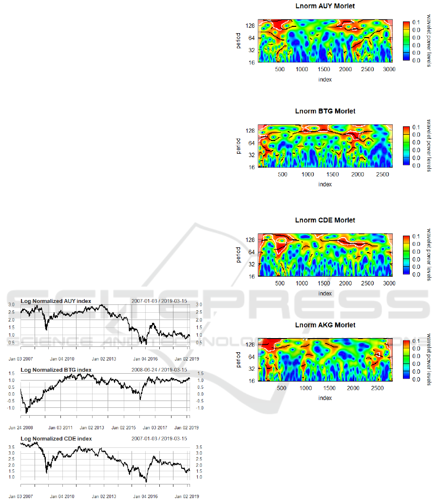
As seen in Figure 1, beginning the analysis with the

gold mining stocks AUY, BTG, CDE, one will im-

mediately recognize that there is a bearish region of

high volatility between 2008 and 2009 which corre-

sponds to the Great Recession. AUY, BTG, CDE re-

cover slightly going into 2010 but then experience a

slow market decline following 2013. Likewise, it is

seen that AUY, BTG, CDE all experience a region

of high volatility and high frequency events similarly

manifesting itself within the Morlet wavelet power

distribution graphs corresponding to the 2008 market

crash in Figures 2 and 3. AUY, BTG and CDE make

a dramatic recovery around 2016 (practically 250%

rise in the case of CDE) which is then reﬂected in

Morlet waveform graphs as high power events across

the lower and middle frequencies. This behavior of

course tapers off as the market ﬁnds resistance and the

Morlet wavelet graphs shift to a lower power level.

Figure 1: Log Normalized Time Series AUY,BTG,CDE.

Similarly to how AUY, BTG, CDE behave, AKG,

EGO and GG in Figure 4 all show a decline in stock

value after 2012 and also exhibit a dip around the

2008. The 2008 decline is most likely indicative of

the effects of the “Great Recession” along with a re-

sulting industry-wide market cool down period fol-

lowing this event. Likewise, AKG, EGO and GG all

exhibit regions of high volatility around the 500 in-

Figure 2: Morlet wavelet power distribution for AUY and

BTG.

Figure 3: Morlet wavelet power distribution for CDE and

AKG.

dex point which directly corresponds to the dramatic

market dip in Figures 3 and 5.

Note that the volatility and high power level re-

gion around index 500 for AKG, EGO and GG is

contrasted with marked decrease in power levels dur-

ing the slight recovery period between 2009 and 2010.

The shift in volatility after index 1000 shows that the

market experiences long periods of cyclic downturn

(illustrated by the long bands of high intensity power

between periods 64 and 120 for indexes 1500-2500).

Periods 64 and 120 correspond to the bimonthly and

quarterly business cycles of these respective ﬁrms.

The long term trading behavior illustrate that the com-

panies were perceived by investors as being worth less

each consecutive quarter; either shorting the market

(long term) or closing their investments.

Data Mining using Morlet Wavelets for Financial Time Series

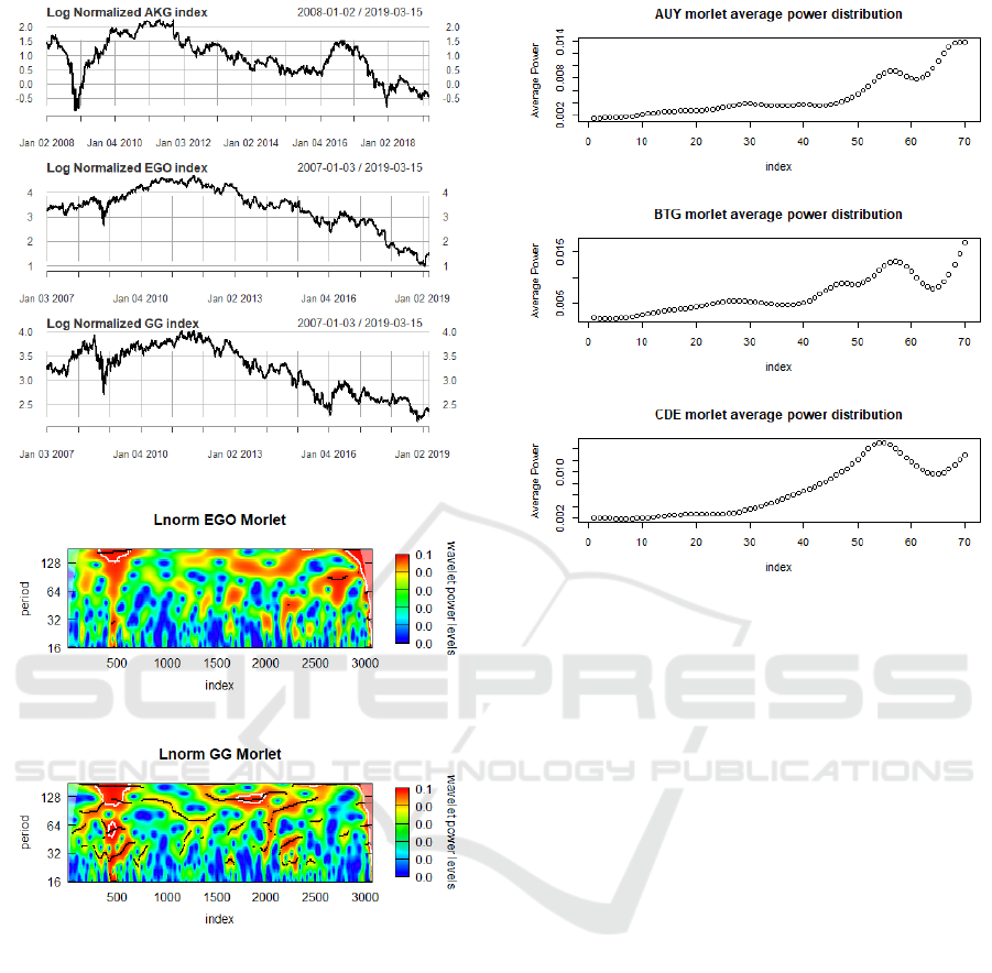
Figure 4: Log normalized Time Series AKG, EGO, GG.

Figure 5: Morlet Wavelet power distribution for EGO and

GG.

After extracting the Morlet wavelet power distri-

bution, the average power over the frequency domain

can be found which is illustrated in Figures 6 and 7.

Surprisingly, it’s clear that the average power in the

frequency domain of the stock indexes EGO and AUY

are almost identical. BTG’s power curve is similar to

either AUY or CDE depending on whether the dip at

index 60 skews the results. It’s hard to discern off

hand where AKG lies with respect to the other power

curves since it’s moving in a more horizontal manner

than GG between the indexes 0-50. AKG appears to

have more volatility than EGO and AUY. This val-

idates our BTSPC algorithm due to the fact that if

stock indexes are more similar to one another then

their power curves will also be similar. In order to

Figure 6: Morlet Wavelet average power at each index of

gold stocks.

measure the amount of similarity between the behav-

ior of a given time series one could sequentially sub-

sample the power curve at a given interval and mea-

sure the distances between each point for a given in-

dex.

After applying the BTSPC algorithm and ﬁnding

the dissimilarity matrix based on the Frechet distances

we then apply the common linkage clustering algo-

rithm. Clustering of the BTSPC data dissimilarity

matrix based on common-linkage method can be seen

in Figure 8. The clustering dendrogram tree shows

two primary clusters forming within the data AUY,

EGO and GG. AUY, EGO and GG are shown to cre-

ate a behavioral block contrasted with the behavior

exhibited by BTG, CDE and AKG. Within the ﬁrst

cluster it is shown that GG behaves independently

to EGO and AUY which is not surprising consider-

ing the dip at index 45 and 65 in GG’s power curve.

Examining the second cluster family, BTG forms a

small cluster with CDE, whereas AKG is left entirely

alone since it is the most dissimilar power distribu-

tion curve. The most similar indexes according to

their average power distributions are AUY, EGO and

surprisingly GG, which form a nice block with one

another. AKG and CDE are shown as the most dis-

similar elements within the sample. Lastly, one can

see that BTG lies at a nice intermediate position be-

tween the behavior of the other indexes which is not

surprising considering the average power distribution

DATA 2019 - 8th International Conference on Data Science, Technology and Applications

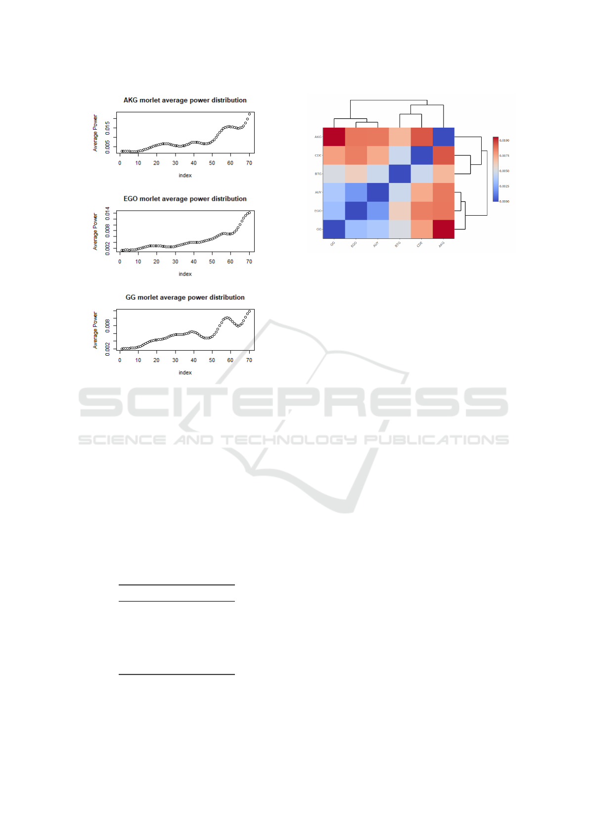
Figure 7: Morlet Wavelet average power at each index of

gold stocks.

curves. Table 1 shows the sorted row averages for

the dissimilarity matrix measured by the Frechet dis-

tance between the motifs. Presumably the increased

volatility in CDE is due to the fact that CDE’s mining

operations are located in Ghana and this might inﬂu-

ence the perception of the company as a whole post

recession. Contrast this with the increased volatility

in AKG which is most likely due to the volatility in

gold markets as a whole but also due to their poor ﬁ-

nancial reports since AKG has been posting year over

year net income losses since 2013 with the exception

of 2016.

Table 1: Frechet Dissimilarity matrix : Sorted by row aver-

ages.

Stock Index Row Averages

AUY 0.004396661

BTG 0.004590316

EGO 0.004772740

GG 0.005036986

CDE 0.006308873

AKG 0.007432775

One can clearly see that Morlet wavelets can be

employed for datamining a given ﬁnancial time se-

ries, since Morlet wavelets essentially allow one to

Figure 8: Common-Linkage Clustering of Morlet wavelet

average power curves.

discover the power distribution patterns with respect

to frequency and time which provides meaningful in-

sight into the underlying behavior of a given econo-

metric system. The BTSPC algorithm demonstrates

that by extracting the average power distribution band

at a given frequency from the Morlet wavelet wave-

form one can then discover the similarities of a given

time series based upon the Frechet distance between

the average power distribution curves. Finally, clus-

tering the resulting dissimilarity matrix allows one to

clearly compare ﬁnancial market indexes with one an-

other in a meaningful manner that provides insight

into how a given industry is behaving.

6 CONCLUSIONS AND FUTURE

WORK

The power of wavelet analysis when applied to time

series datamining is the capability of representing the

range of high/low frequency components and the in-

tensity/distribution of these frequency components as

a function of time. This allows one the ability to to

pick out cylical trends at different time resolutions

in a single procedure compared with the traditional

method having to spend hours optimizing a time win-

dow interval iteratively.

With the Morlet wavelet speciﬁcally, it has been

shown that the waveform resulting from the Morlet

wavelet function is able to discover the exact frequen-

cies at which dominant trading behavior occurs across

time which can be used in order to visualize the evo-

lution of trading behaviors. This is a fundamentally

different approach to traditional econometric analysis

methods as one is able to both visualize the trend of

a market and simultaneously the volatility and cycli-

cal components of the market using only the Morlet

Data Mining using Morlet Wavelets for Financial Time Series

wavelet. The BTSPC algorithm capitalizes on this

fact and is able to then create a piecewise comparison

between the trading behaviors of the stock indexes

across all frequency ranges and across time avoiding

the problems of resolution which were inherent to tra-

ditional DFT analysis methods. Further, the BTSPC

cluster results create a dynamic image of the mar-

ket behavior in question which yields itself to data

driven analysis approach due to the fact that the al-

gorithm utilizes Morlet wavelets. Consequently, the

BTSPC method is vastly superior for analyzing poten-

tially thousands of market indexes compared with tra-

ditional analysis approaches which require active user

guidance such as ARIMA, neural networks or Fourier

transforms. Finally, unlike ARIMA, neural networks

and Fourier transform analysis, it’s important to note

that data analyzed by BTSPC requires no data pre-

processing (transformations to linearity, forcing sta-

tionarity via differencing, etc) which vastly simpliﬁes

any given macro-economic analysis.

In this study, it was discovered that all of the

gold mining ﬁrms (AUY, BTG, CDE, AKG, EGO,

GG) exhibited increased high-frequency activity dur-

ing the recessionary period of 2008 followed by a

brief low-frequency/low intensity recovery phase un-

til 2013 when the stock prices across all indexes in

the study began declining. The BTSPC algorithm was

utilized to compare the motifs contained within the re-

spective time series by constructing a matrix of power

curves. It was then found that the gold mining ﬁrms

in this study formed two cluster families AUY, EGO

and GG and BTG, CDE, AKG. It was also shown that

CDE and AKG are the most dissimilar time series

in the analysis which is due to the more pronounced

volatility contained within the individual series itself.

It is speculated that the increased volatility is in part

due to the perception that CDE and AKG both may be

perceived as risky investments and negative investor

sentiment is therefore inﬂuencing these indexes.

Future work could include testing the BTSPC al-

gorithm to different market sectors in order to form a

broader understanding of trading behavior. Since the

BTSPC can be utilized to provide qualitative and pre-

dictive information from any two (or more) signals,

any situations where there exists two or more concur-

rent dynamic processes within a macro-process the

BTSPC can be utilized in order to dynamically ana-

lyze how these processes behave with respect to one

another within the framework of the macro-process

itself. For example, if we know that two or more

stock indexes currently exhibit similarity (aka co-

movement) as evidenced by the BTSPC algorithm and

clustering then one can predict radical cross-market

changes by merely examining whatever stock begins

to diverge from the other stocks in the analysis. Thus,

one can use the BTSPC to creating a dynamic or real

time visualization of market dynamics for investors

and ﬁnancial institutions. Similarly, one could extend

the BTSPC algorithm to examinations of emergent

behavior in ecology, meteorological applications, bi-

ological systems, etc. Finally, BTSPC could be ap-

plied to social media data mining and search result

optimization as it would allow one to visualize the

differences between keywords across frequencies and

time which would provide information about user be-

havior. The applications of the BTSPC algorithm are

limitless.

REFERENCES

Aguiar-Conraria, L., Azevedo, N., and Soares, M. J. (2008).

Using wavelets to decompose the time–frequency ef-

fects of monetary policy. Physica A: Statistical me-

chanics and its Applications, 387(12):2863–2878.

Choudhary, M. A. and Haider, A. (2012). Neural network

models for inﬂation forecasting: an appraisal. Applied

Economics, 44(20):2631–2635.

Defays, D. (1977). An efﬁcient algorithm for a complete

link method. The Computer Journal, 20(4):364–366.

Dowson, D. and Landau, B. (1982). The fr

echet distance

between multivariate normal distributions. Journal of

multivariate analysis, 12(3):450–455.

Ehlers, J. F. (2007). Fourier transform for traders. TECHNI-

CAL ANALYSIS OF STOCKS AND COMMODITIES-

MAGAZINE EDITION-, 25(1):24.

Fahimifard, S., Homayounifar, M., Sabouhi, M., and

Moghaddamnia, A. (2009). Comparison of anﬁs, ann,

garch and arima techniques to exchange rate forecast-

ing. Journal of Applied Sciences, 9(20):3641–3651.

Gallegati, M., Ramsey, J. B., and Semmler, W. (2014). In-

terest rate spreads and output: A time scale decompo-

sition analysis using wavelets. Computational Statis-

tics & Data Analysis, 76:283–290.

Goupillaud, P., Grossmann, A., and Morlet, J. (1984).

Cycle-octave and related transforms in seismic signal

analysis. Geoexploration, 23(1):85–102.

Huang, C., Huang, L.-l., and Han, T.-t. (2012). Financial

time series forecasting based on wavelet kernel sup-

port vector machine. In 2012 8th International Con-

ference on Natural Computation, pages 79–83. IEEE.

Huang, J.-N., Li, H., Maechler, M., Martin, R. D., and

Schimert, J. (1992). A comparison of projection

pursuit and neural network regression modeling. In

Advances in Neural Information Processing Systems,

pages 1159–1166.

Leybourne, S. J., McCabe, B. P., and Tremayne, A. R.

(1996). Can economic time series be differenced to

stationarity? Journal of Business & Economic Statis-

tics, 14(4):435–446.

Richette, P., Clerson, P., P

erissin, L., Flipo, R.-M., and

Bardin, T. (2015). Revisiting comorbidities in gout:

DATA 2019 - 8th International Conference on Data Science, Technology and Applications

a cluster analysis. Annals of the rheumatic diseases,

74(1):142–147.

Symeonidis, P., Iakovidou, N., Mantas, N., and Manolopou-

los, Y. (2013). From biological to social networks:

Link prediction based on multi-way spectral cluster-

ing. Data & Knowledge Engineering, 87:226–242.

Data Mining using Morlet Wavelets for Financial Time Series