Modeling Dynamic Processes with Deep Neural Networks: A Case Study

with a Gas-ﬁred Absorption Heat Pump

Jens Lippel, Martin Becker and Thomas Zielke

University of Applied Sciences D

usseldorf, M

unsterstr. 156, 40476, D

usseldorf, Germany

Keywords:

Deep Neural Networks, Machine Learning, Dynamic Processes, Gas-ﬁred Absorption Heat Pump, Simulation,

Modeling.

Abstract:

Deriving mathematical models for the simulation of dynamic processes is costly and time-consuming. This

paper examines the possibilities of deep neural networks (DNNs) as a means to facilitate and accelerate this

step in development. DNNs are machine learning models that have become a state-of-the-art solution to a

wide range of data analysis and pattern recognition tasks. Unlike mathematical modeling approaches, DNN

approaches require little to no domain-speciﬁc knowledge. Given a sufﬁcient amount of data, a model of the

complex nonlinear input-to-output relations of a dynamic system can be learned autonomously. To validate

this DNN based modeling approach, we use the example of a gas-ﬁred absorption heat pump. The DNN is

learned based on several measurement series recorded during a hardware-in-the-loop (HiL) simulation of the

heat pump. A mathematical reference model of the heat pump that was tested in the same HiL environment is

used for a comparison of a mathematical and a DNN based modeling approach. Our results show that DNNs

can yield models that are comparable to the reference model. The presented methodology covers the data

preprocessing, the learning of the models and their validation. It can be easily transferred to more complex

dynamic processes.

1 INTRODUCTION

Heat pumps are complex nonlinear dynamic systems

with several input and output variables. It has long

been known that artiﬁcial neural networks (ANNs)

are suited for the empirical modeling of such systems

(Carriere and Hamam, 1992). The modeling is based

on measurements of the input and output variables of

a real system in its relevant operation conditions and

can often be realized without any prior knowledge

about the system behavior. An ANN uses the mea-

surements to approximate the system behavior with

the help of a learning algorithm. While (Carriere and

Hamam, 1992) used the learned model to design a

controller, the more general modeling goal is often

the continuous analysis of the system behavior with

respect to a speciﬁed scope per input variable – this

includes the modeling of system states not explicitly

reﬂected by the given set of measurements (Bechtler

et al., 2001) (Wang et al., 2013).

The ANN based modeling approach is often only

carried out without considering the system’s dynamic

behavior (cf. (Bechtler et al., 2001), (Shen et al.,

2015), (Ledesma and Belman-Flores, 2016), (Reich

et al., 2017)). In this case, the measurement of the

input and output variables at a given point in time is

treated as temporally isolated, i.e. it is not viewed in

relation with its temporally adjacent measurements.

One way to realize a time series based learning is to

use so-called recurrent neural networks (Frey et al.,

2011) (Kose and Petlenkov, 2016). Another way is to

extract temporal features from the time series and use

them as additional input variables for the learning of

an ANN (Le Guennec et al., 2016).

In this paper, we describe two approaches to the

extraction of temporal features. These features serve

as additional input variables for the learning of large

multilayer ANNs, so-called deep neural networks

(DNNs) (Stuhlsatz et al., 2010). We consider a gas-

ﬁred absorption heat pump as an exemplary dynamic

system. However, the described temporal feature ex-

traction, the subsequent learning of DNNs and the ﬁ-

nal validation of the resulting models are applicable to

any dynamic system with continuous input and output

variables.

1.1 Database and Objective

The measured data that form the basis of the DNN

based modeling approach have been recorded dur-

Lippel, J., Becker, M. and Zielke, T.

Modeling Dynamic Processes with Deep Neural Networks: A Case Study with a Gas-ﬁred Absorption Heat Pump.

DOI: 10.5220/0007932903170326

In Proceedings of the 9th International Conference on Simulation and Modeling Methodologies, Technologies and Applications (SIMULTECH 2019), pages 317-326

ISBN: 978-989-758-381-0

317

h,out

condenser / absorber

evaporator

heat accumulator

heating circuit

gas

h,in

c,in

c,out

cold water circuit

cold water reservoir

external cooling

internal circuit

gas-ﬁred

absorption

heat pump

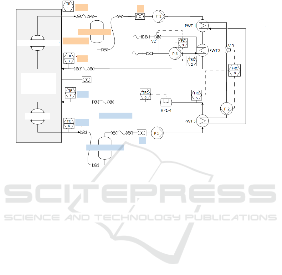
Figure 1: Hydraulic circuit diagram of the hardware-in-the-loop (HiL) test bench. It was used to run all simulations. During

the simulations the input variables

gas

, T

h,in

, T

c,in

and

as well as the output variables T

h,out

and T

c,out

were recorded

with a sample frequency of 1 Hz over a period of 25 days.

ing a hardware-in-the-loop (HiL) simulation of the

considered heat pump; a Buderus GWPW41 with

an ammonia-water absorption cycle. The heat pump

is operated as a system component in a realistically

modeled environment. It interacts with other system

components and reacts to simulated weather condi-

tions as well as a simulated user behavior. The HiL

test bench functions as a coupling point between the

simulation (interface connection) and the hardware

(hydraulically connected). The system’s outlet ﬂow

temperature is passed to the simulation via its inter-

face connection. Then, the return ﬂow temperature is

simulated and passed back to the test bench, where

it serves as a set point for the regulation of the ﬂuid

ﬂows that enter the heat pump.

A hydraulic circuit diagram of the HiL test bench

is depicted in Figure 1. The annotations show where

the input variables

•

gas

/h]: volume ﬂow rate of used gas

• T

h,in

[

◦

C]: inlet temperature (heating circuit)

• T

c,in

[

◦

C]: inlet temperature (cold water circuit)

•

/h]: volume ﬂow rate (heating circuit)

•

/h]: volume ﬂow rate (cold water circuit)

and the output variables

• T

h,out

[

◦

C]: outlet temperature (heating circuit)

• T

c,out

[

◦

C]: outlet temperature (cold water circuit)

of the heat pump are measured.

The goal of our research is to learn a DNN that is

capable of predicting the output variables of the heat

pump when given its input variables. To this end, we

have access to several measurement series. Each was

recorded at a sample frequency of 1 Hz. The overall

data set includes about 25 days of measurements and

covers all relevant operation conditions. More details

on the data set are given in Section 2.4.

To assess the prediction accuracy of the learned

model, we compare it with the mathematical model

presented by (Goebel et al., 2015). Their modeling

is not based on the chemical and physical processes

of the heat pump as this leads to an overly complex

model and a long simulation time. Instead, they used

characteristic diagrams that represent sufﬁciently ac-

curate look-up tables for the modeling of the input-

to-output relations of the heat pump. This model was

validated with the above measurement series and it

is therefore well suited as a reference model for the

DNN based model.

To further show that too simple machine learning

methods are less suited than DNNs, we also applied a

multivariable linear regression (Duda et al., 2001) to

obtain prediction models (cf. Section 3).

SIMULTECH 2019 - 9th International Conference on Simulation and Modeling Methodologies, Technologies and Applications

318

h,out

(t)

gas

(t)

h,in

(t)

c,in

(t)

input neurons hidden neurons

output neuron

raw features

temporal features

∑

t∈Φ

h,out

(t) − T

h,out

(t)|

Φ := random set of observation times

h,out

:= predicted output

h,out

:= measured output

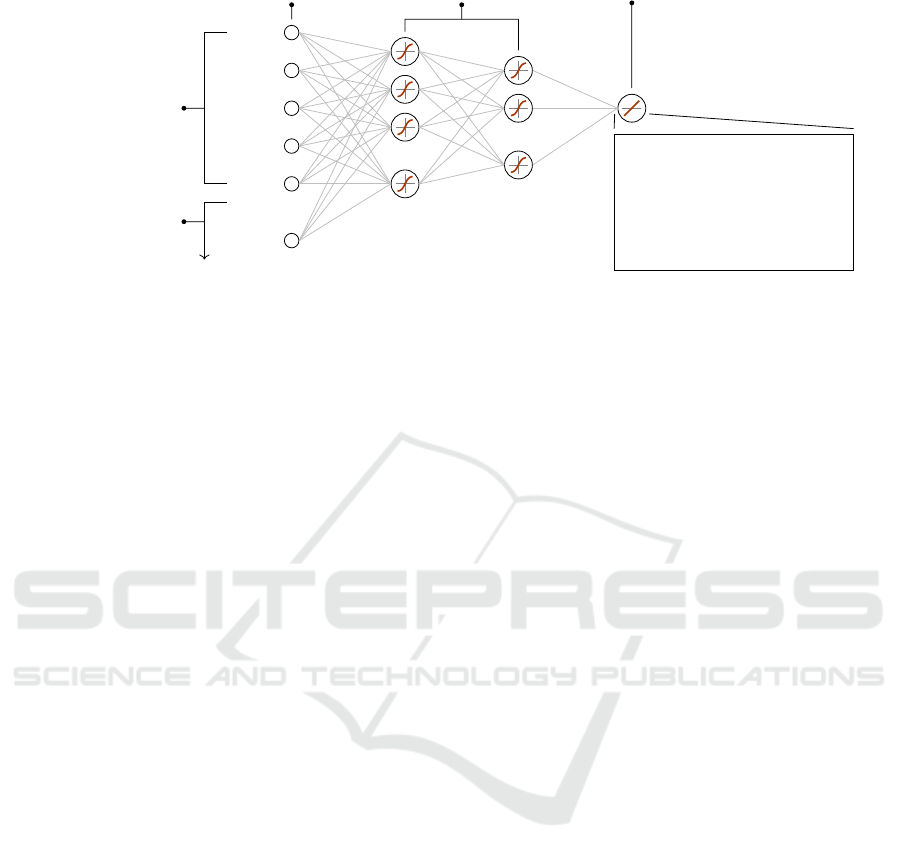
Figure 2: General structure of a DNN. A DNN consists of several layers of artiﬁcial neurons. The original, non-preprocessed

measurements of the input variables (raw features) are fed into the DNN via input neurons. The same applies to the extracted

temporal features (i.e. the results of the data preprocessing with Method A or B). Each of the features is fed into a separate

input neuron. The ﬁnal prediction is generated through at least two layers of hidden neurons and one output neuron. The

DNN’s optimization is carried out with respect to the loss stated in the lower right box.

Regarding the comparison of the learned models

and the reference model, it is important to note that

all simulations were carried out in a cyclic operation

mode where the cold water circuit was switched off

during the deactivation phase of a cycle. During this

phase, the used simulation does not provide accurate

temperatures. However, they quickly become accu-

rate once the cold water circuit has been switched on

again. In (Goebel et al., 2015), the validation of the

model is therefore not based on measurements where

(t) 6= 0. In our research, these measurement peri-

ods are not considered for the same reason: They are

neither used for the learning of models nor for their

validation. As a result, the effective data set size had

to be reduced to approximately 12 days (of originally

25 days) of measurements.

1.2 Deep Neural Networks

ANNs, and especially DNNs, have been shown to be

powerful parametric machine learning models. One

main advantage of DNNs is that there exists a wide

range of learning algorithms that carry out an efﬁcient

and automatic parameter optimization. An adaption

of these learning algorithms to the concrete learning

task at hand is often not necessary and it is therefore

generally not required to fully understand the princi-

ples that they are based on.

In this work, we use a slightly modiﬁed version

of a DNN called ReNDA, a Regularized Nonlinear

Discriminant Analysis (Becker et al., 2017). So far,

this DNN and its predecessor GerDA (Generalized

Discriminant Analysis) have primarily been used to

solve classiﬁcation tasks (cf. (Gaida et al., 2012),

(Stuhlsatz et al., 2012)). In the course of this work,

we extended ReNDA so that it can be applied to mul-

tivariable nonlinear regression tasks. This allowed

us to learn the desired prediction model. Our exten-

sion preserves the preoptimization strategy described

in (Stuhlsatz et al., 2012). It is a measure that has

been shown to decrease the risk of converging towards

poor local optima in the DNN’s parameter space (Er-

han et al., 2010).

2 METHODOLOGY

As mentioned in the introduction, one way to realize

the time series based learning of a DNN is to extract

temporal features from the time series and use them

as additional input variables. Suitable approaches to

the extraction of temporal features are usually based

on prior knowledge about the application at hand. In

most scenarios, acquiring this knowledge goes hand

in hand with planning the recording of the data. At

a later time, the initial approaches can be gradually

improved based on own results, or results from other

researchers.

In the following, we describe two quite differ-

ent approaches to extracting temporal features. Here

and subsequently, we refer to them as Method A and

Method B. They can both be understood as a form

of data preprocessing that has to be carried out be-

fore the actual learning of a DNN. The features result-

ing from this data preprocessing are fed into a DNN’s

input neurons along with the non-preprocessed mea-

surements (also called raw features). As can be seen

in Figure 2, each feature is fed into a separate input

neuron.

Figure 2 also shows the structure of a DNN and

states the loss function that is used to optimize it. In

Modeling Dynamic Processes with Deep Neural Networks: A Case Study with a Gas-ﬁred Absorption Heat Pump

319

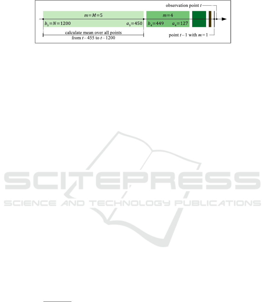
Figure 3: Graphical explanation of the averaged past values (APVs) as deﬁned by (2). The displayed example for N = 1200

and M = 5 is also used as a setup in our experiments (cf. Section 3.1).

Section 2.3, we give a brief explanation of these two

aspects (cf. (Becker et al., 2017) for further details).

Moreover, we introduce two different metrics for the

validation of the learned prediction models.

2.1 Method A: Time Series

Representation

Because heat pumps are dynamic systems, predicting

h,out

(t) and T

c,out

(t) based on the already measured

time series of its input variables; namely

gas

(t − n),

h,in

(t − n), T

c,in

(t − n),

(t − n) and

(t − n) for

n ∈ {0,1,.. .,N} with N ≥ 0; is reasonable. In this

way, we consider the measurements at observation

time (n = 0) and N past measurements (1 ≤ n ≤ N).

In the case of ReNDA and most other DNNs, N has to

be constant during the entire learning process, i.e. the

time series must be of equal length. Assuming that

the ﬁrst sample of a time series has the index 1, the

ﬁrst possible time series of length N corresponds to

the observation time t = N + 1.

A second reasonable assumption is that measure-

ments of the input variables in the closer past (n ≈ t)

have a more direct effect on T

h,out

(t) and T

c,out

(t) than

those of the distant past (n  t). Because this is true

for a wide range of dynamic systems, we developed

the following general method for the extraction of

temporal features from a time series of length N: Let

m ∈ {1,2,.. ., M} with M ≤ N and let

:= b(m − 1)

c + 1

:= bm

(1)

with γ := log

(N). We call each

gas

(t) :=

− a

+ 1

∑

n=a

gas

(t − n) (2)

an averaged past value (APV) of

gas

. See Figure 3

for a graphical explanation. The following holds for

the resulting M APVs:

•

gas

(t) =

gas

(t − 1) since a

= 1 = b

•

gas

(t) includes

gas

(t − N) since b

= N.

• All M intervals [b

] are non-overlapping since

6= b

m−1

for all m ∈ {2,3,.. ., M}.

•

gas

(t) =

gas

(t − m) for all m ∈ {1, 2,. .. ,M} if

M = N, i.e.

gas

(t) is the original time series.

• The index m can be seen as a replacement of the

original time index n.

The APVs T

h,in

, T

c,in

and

of the other input

variables are computed analogously and thus share

the above properties. Since we consider a total of 5

input variables, feeding both the raw features and the

APVs into a DNN requires 5 · (1 + M) input neurons

(cf. Figure 2).

Clearly, the above APV deﬁnition can be easily

applied to any time series of length N, i.e. it is not

limited to the considered heat pump scenario. In the

next section, we describe an alternative method that

relies on expert knowledge about the examined heat

pump.

2.2 Method B: Deﬁnition of a Status of

the Heat Pump

Generally applicable methods like the one described

in the previous section are especially helpful if there

exists no knowledge about a given application. In the

following, we deﬁne a temporal feature representing

the status of the heat pump. By means of this status,

we demonstrate the use of expert knowledge based

temporal features.

Let S

denote the status of the heat pump. It is

deﬁned as follows:

• If the gas burner is switched on at an observation

time t, the sign of S

(t) is positive. Otherwise,

the sign is chosen to be negative.

• The absolute value of S

(t) indicates the period

of time for which the gas burner has already been

in its current state; either switched on or off.

• S

is measured in seconds.

For instance, if the gas burner has been switched off

for 5 seconds at observation time t, the status of the

heat pump is S

(t) = −5s.

Note that using S

requires a ﬁxed number of 6

input neurons as opposed to a minimum number of

5 · (1 + M) = 10 for M = 1 in Method A. Note also

SIMULTECH 2019 - 9th International Conference on Simulation and Modeling Methodologies, Technologies and Applications

320

that choosing M = 1 yields a rather unsophisticated

representation of a time series: the average of all N

past values. Therefore, it is recommended to choose

M > 1, which implies the use of a DNN with 15 or

more input neurons. Consequently, Method B leads

to a signiﬁcantly lower computational effort during

the learning of a DNN.

2.3 Model Optimization and Feature

Processing

Once Method A or B has been applied to extract tem-

poral features, each raw and each temporal feature is

fed into its respective input neuron. Then, a layered

structure of hidden neurons followed by one output

neuron generates a prediction (cf. Figure 2). Although

it is generally possible to use multiple output neurons,

we choose to learn one DNN per output variable (i.e.

separate prediction models for T

h,out

and T

c,out

). The

intuition behind this is that it is easier for a DNN to

adapt itself to only one output variable. Studying a

DNNs capability to simultaneously adapt to two or

more output variables is subject to future work.

Subsequently, we give a brief explanation on how

a DNN is optimized and how it processes features. To

improve clarity, we focus on the DNN for T

h,out

; the

explanation is also valid for T

c,out

As stated in Figure 2, the optimization of a DNN

is based on a loss given by

∑

t∈Φ



h,out

(t) − T

h,out

(t)



(3)

where Φ is a random set of observation times. First,

the DNN generates the predictions

h,out

(t), which is

done by processing the respective raw and temporal

features. The above loss and its derivative are then

used to realize a gradient descent based update of all

parameters of the DNN. These two steps are carried

out for several random sets Φ until the loss becomes

sufﬁciently small.

The parameters updated during this optimization

are the adjustable weights and biases of the hidden

neurons and the output neuron. Each individual neu-

ron processes its input signals x

via



b +

∑

· x



(4)

where f is called an activation function, b is called a

bias and each w

is called a weight. In our case, f is

deﬁned by f (ξ) := sigm(ξ) := 1/(1 + exp(−ξ)) for

each hidden and by f (ξ) := ξ for the output neuron.

While the search of suitable activation functions is a

hot topic (Basirat and Roth, 2018), practitioners can

often already achieve good learning results by choos-

ing an appropriate DNN topology (the number of lay-

ers of hidden neurons and the number of neurons per

layer). The DNN topology ultimately determines the

overall number of adjustable weights and biases of a

DNN; it therefore represents the number of degrees

of freedom that can be used to learn a good prediction

model.

2.4 Model Validation

In addition to the loss (3), we consider two different

metrics to measure the goodness of the learned pre-

diction models. One is the relative error

err

rel

|Φ|

∑

t∈Φ



h,out

(t)

h,out

(t)

− 1



· 100% (5)

where |Φ| denotes the number of randomly selected

observation times. The other is the absolute error

err

abs

|Φ|

∑

t∈Φ

h,out

(t) − T

h,out

(t)|. (6)

In the case of both metrics, we used

h,out

and T

h,out

◦

C. For lowest values of ≈ 3

◦

C, we experienced

no numerical issues when calculating (5); here, a di-

vision through 0

◦

C would have been problematic. In

the case of err

abs

, all results are stated in Kelvin (K)

as it is common with temperature differences.

The ultimate goal of any machine learning based

modeling approach is to learn a model that performs

well on unseen data (e.g. future measurements). It is

therefore necessary to split the data into training and

validation data. Learning a model, i.e. updating its

parameters, is solely based on the training data. The

validation data, on the other hand, simulates unseen

data that does not serve as a learning basis. It is only

used to monitor the learning process and, especially,

to prevent the learning of an overﬁtted model (Tetko

et al., 1995).

In our experiments, we consider the 3 data pack-

ages (DP1 to DP3) speciﬁed in Table 1. To simulate

unseen data in the most realistic way, the validation

data of each data package comes from exactly 1 of 6

mutually independent measurement series. To speed

up the DNN learning process, we use 400,000 ran-

domly selected measurements from the remaining 5

measurement series as training data. This amount of

training data proved to be sufﬁcient for the learning of

a prediction model (i.e. the learning led to a gradual

improvement of the model). Using 3 data packages

enables us to compare the learning performance un-

der different training conditions.

Modeling Dynamic Processes with Deep Neural Networks: A Case Study with a Gas-ﬁred Absorption Heat Pump

321

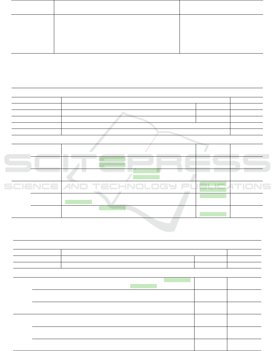
Table 1: Deﬁnition of different data packages. Each consists of different training and validation samples. For the partitioning

of the data into sets of training and validation samples, we simply used the IDs of the measurement series. In the case of all

data packages, the validation is based on 1 of 6 mutually independent measurement series that was not used for the learning

of the DNN. This realistically simulates unseen data for a proper model validation (cf. Section 2.4).

Data package Training data Validation data

Measurement series ID No. of measurements meas. series ID No. of meas.

DP1 321; 324; 350; 351; 353 548,771

∗

319 485,339

DP2 319; 324; 350; 351; 353 562,113

∗

321 471,997

DP3 321; 321; 350; 351; 353 969,207

∗

324 64,903

∗

) To speed up the learning process, we only

use 400,000 randomly sampled measurements.

Table 2: Average relative and absolute errors and the corresponding standard deviation of the predictions obtained from

different DNN based models. The last column shows the comparative results obtained from the reference model (Goebel

et al., 2015). The results highlighted in bold are the best result within this table. The results highlighted in green are the best

results within this table and Table 3.

Experimental setup

Model DNN Reference

Data preprocessing Method A Method B N/A

M in Eq. (2) 3 5 10 20 N/A N/A

Input neurons 20 30 55 105 6 N/A

Hidden neurons 3 layers with 50, 25 and 100 neurons, respectively N/A

Output neurons 1 neuron since we chose to learn one DNN per output variable N/A

Results

h,out

DP1

% 0.87 ± 1.61 0.80 ± 1.38 0.97 ± 1.26 1.26 ± 1.79 0.75 ± 1.17 0.88 ± 2.48

K 0.37 ± 0.63 0.35 ± 0.46 0.42 ± 0.43 0.56 ± 0.53 0.31 ± 0.37 0.35 ± 0.91

DP2

% 0.48 ± 0.98 0.37 ± 0.65 0.48 ± 0.84 0.93 ± 1.31 0.66 ± 1.18 1.08 ± 2.71

K 0.20 ± 0.33 0.16 ± 0.21 0.21 ± 0.23 0.43 ± 0.43 0.28 ± 0.42 0.45 ± 1.08

DP3

% 0.64 ± 1.57 0.54 ± 1.25 0.50 ± 0.92 0.59 ± 1.23 0.69 ± 1.71 1.44 ± 2.98

K 0.23 ± 0.44 0.19 ± 0.34 0.18 ± 0.22 0.21 ± 0.31 0.25 ± 0.61 0.48 ± 0.79

c,out

DP1

% 2.05 ± 3.60 1.84 ± 3.02 2.55 ± 4.51 5.60 ± 7.01 1.33 ± 2.12 2.10 ± 5.23

K 0.18 ± 0.34 0.16 ± 0.25 0.22 ± 0.44 0.46 ± 0.46 0.12 ± 0.19 0.17 ± 0.31

DP2

% 1.06 ± 2.29 1.18 ± 1.72 1.65 ± 2.18 4.00 ± 6.10 1.05 ± 1.78 2.09 ± 6.47

K 0.09 ± 0.14 0.10 ± 0.13 0.14 ± 0.19 0.31 ± 0.37 0.10 ± 0.16 0.16 ± 0.37

DP3

% 0.92 ± 2.00 0.87 ± 1.83 1.04 ± 2.77 1.65 ± 3.88 0.93 ± 2.54 1.08 ± 2.27

K 0.13 ± 0.34 0.12 ± 0.36 0.15 ± 0.57 0.23 ± 0.73 0.12 ± 0.27 0.16 ± 0.39

Table 3: Average relative and absolute errors and the corresponding standard deviation of the predictions obtained from

different multivariable linear regression models. The table is organized and designed as Table 2.

Experimental setup

Model Multivariable linear regression Reference

Data reprocessing Method A Method B N/A

M in Eq. (2) 3 5 10 20 N/A N/A

Results

h,out

DP1

% 1.35 ± 1.84 0.52 ± 0.89 0.45 ± 0.87 0.45 ± 0.85 1.39 ± 2.70 0.88 ± 2.48

K 0.59 ± 0.72 0.22 ± 0.35 0.19 ± 0.34 0.20 ± 0.33 0.57 ± 0.97 0.35 ± 0.91

DP2

% 1.25 ± 1.95 0.55 ± 0.83 0.52 ± 0.76 0.51 ± 0.74 1.96 ± 2.90 1.08 ± 2.71

K 0.53 ± 0.76 0.25 ± 0.30 0.24 ± 0.27 0.23 ± 0.26 0.84 ± 1.02 0.45 ± 1.08

DP3

% 2.42 ± 3.38 0.95 ± 1.74 0.86 ± 1.64 0.85 ± 1.62 3.50 ± 5.31 1.44 ± 2.98

K 0.90 ± 1.17 0.34 ± 0.53 0.31 ± 0.49 0.31 ± 0.49 1.27 ± 1.67 0.48 ± 0.79

c,out

DP1

% 4.15 ± 3.58 2.54 ± 2.05 2.36 ± 1.96 2.47 ± 1.97 3.30 ± 4.33 2.10 ± 5.23

K 0.34 ± 0.32 0.21 ± 0.19 0.19 ± 0.18 0.20 ± 0.18 0.29 ± 0.41 0.17 ± 0.31

DP2

% 2.70 ± 3.59 1.63 ± 1.99 1.60 ± 1.91 1.58 ± 1.90 4.30 ± 4.60 2.09 ± 6.47

K 0.23 ± 0.33 0.13 ± 0.17 0.12 ± 0.16 0.12 ± 0.16 0.35 ± 0.43 0.16 ± 0.37

DP3

% 3.16 ± 3.93 1.30 ± 1.96 1.21 ± 1.85 1.20 ± 1.84 4.18 ± 5.42 1.08 ± 2.27

K 0.39 ± 0.53 0.17 ± 0.35 0.16 ± 0.34 0.16 ± 0.33 0.52 ± 0.70 0.16 ± 0.39

SIMULTECH 2019 - 9th International Conference on Simulation and Modeling Methodologies, Technologies and Applications

322

3 EXPERIMENTS

In this section, we present the setup and results of a

series of experiments that we carried out in order to

ﬁnd answers to the following questions:

• Are the proposed data preprocessings (Method A

and B) suitable for the DNN based modeling of

dynamic systems?

• Does the DNN based approach yield models that

are comparable with the reference model (Goebel

et al., 2015)?

• How does the number M of APVs (Method A,

cf. Section 2.1, Eq. (2)) effect the accuracy of the

learned prediction model?

• How do the learned models compare with simple

multivariable linear regression models?

3.1 Experimental Setup and Average

Results

In general, the successful DNN based modeling of

a dynamic system depends on various DNN-speciﬁc

hyperparameters. The most relevant are stated in the

experimental setup subtable of Table 2. We consider

Method A (for N = 1200 and 4 different numbers of

APVs) and Method B with a common layered struc-

ture of hidden and output neurons. Since we deﬁned

3 data packages (Table 1) and chose to learn separate

models for T

h,out

and T

c,out

, we see the results of 30

experiments. The results obtained with the reference

model are stated in the last column of Table 2. In all

cases, the average relative and absolute error and the

associated standard deviations are based on the vali-

dation data of the respective data package. The best

result – the minimum average error – of each row is

highlighted in bold.

Concerning our ﬁrst question, we see that there is

always at least one concrete data prepocessing strat-

egy for which the DNN outperforms the reference

model. This already answers the second question. In

the case of the third question, we can only observe a

slight tendency: In almost all rows, the relative and

absolute error become larger as M increases.

Table 3 helps us to answer the fourth question. It

shows comparative results of 30 multivariable linear

regression models that are based on the exact same

data processing setups as the DNN based models. It is

organized as Table 2 – the last column of Table 2 and

Table 3 are identical. To facilitate a comparison of

Table 2 and Table 3, the green highlightings mark the

best overall results. The multivariable linear regres-

sion models for the prediction of T

h,out

whose model

parameters are based on DP1 (Method A with either

M = 10 or M = 20) are the only models that outper-

form the corresponding DNN based models.

Going beyond the four questions posed, there are

further interesting aspects to discover in Table 3. As

can be seen, the reference model appears to perform

better in three cases. Observe however, that the cor-

responding standard deviations are quite large. It is

therefore likely that the multivariable linear regres-

sion models learned a better time series approxima-

tion of their respective output variable.

3.2 Time Series Approximation Results

While average results provide a good overview over

the suitability of a large number of models, they fail

to reﬂect a model’s power to accurately approximate

output variables that represent time series.

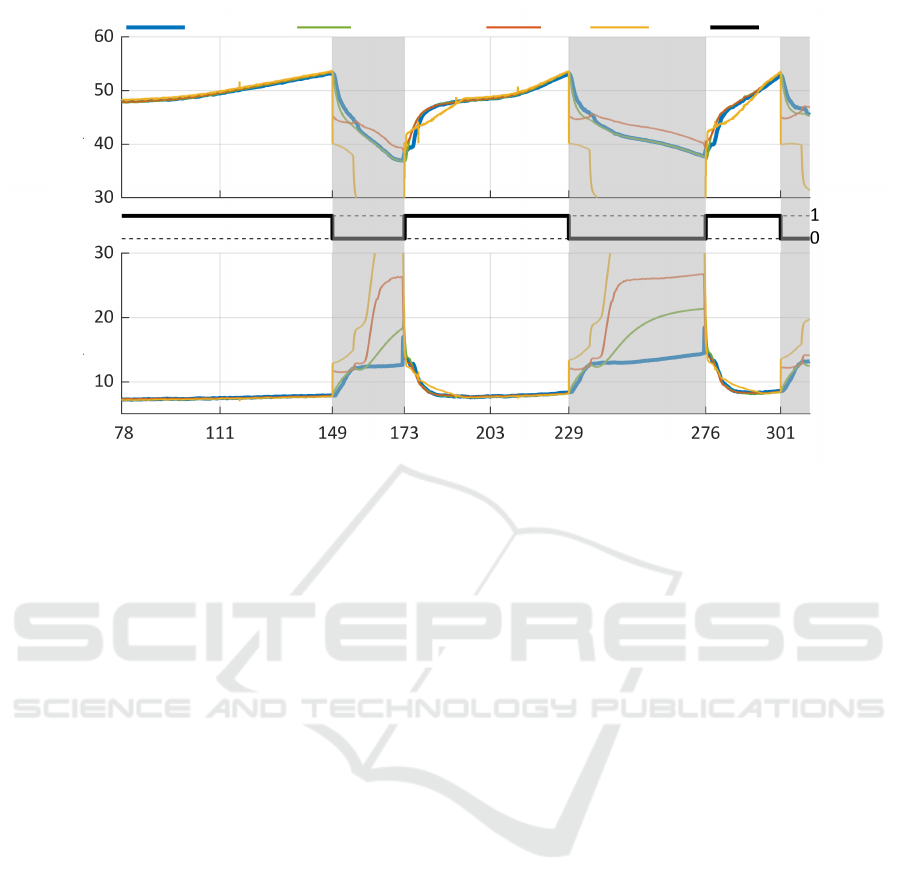
Figure 4 shows a short time series snippet of both

h,out

and T

c,out

. The snippet covers about 4 hours of

measurements and predictions; the latter come from

the DNN model and the multivariable linear regres-

sion model whose parameters are based on features

extracted with Method B (cf. Section 2.2). Both the

reference model and the DNN based model yield an

accurate approximation of T

h,out

and T

c,out

during the

activation phases (

(t) 6= 0). Because the learning of

the DNN is only based on activation phase measure-

ments (cf. Section 1.1), the approximation is signiﬁ-

cantly less accurate during the displayed deactivation

phases (gray highlighted areas). This behavior is es-

pecially pronounced in the case of the multivariable

linear regression model. However, all three models

improve towards the end of an activation phase. The

small outliers of the graph of the multivariable linear

regression model predictions appear to occur at ran-

dom and most likely come from rounding errors. An

analysis of this effect is part of our future research.

A natural question that arises when studying Fig-

ure 4 is the following:

• Which of the three models performs best shortly

after the reactivation of the heat pump (i.e. at the

beginning of each activation phase)?

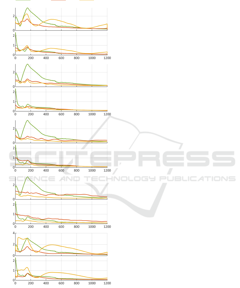
Figure 5 shows our ﬁrst idea on how to approach the

above question. To get a statistically signiﬁcant esti-

mate of the average post-activation-behavior of each

model, we consider the validation data of all 3 data

packages DP1 to DP3. Together, they contain a total

number of 549 activation events. Based on these 549

events, we extracted 549 time frames covering up to

1200 seconds after an activation event. In the case of

an activation duration shorter than 1200 seconds, the

corresponding time frame is limited to the respective

activation duration. Each graph depicted in Figure 5

Modeling Dynamic Processes with Deep Neural Networks: A Case Study with a Gas-ﬁred Absorption Heat Pump

323

temperature in

◦

Ctemperature in

◦

measurement

reference model

DNN

lin.reg.

6= 0

time after last activation in minutes

Figure 4: Short time series snippet of measurements and predictions – T

h,out

and

h,out

(top); T

c,out

and

c,out

(bottom). The

predictions come from the reference model (green), the DNN based model (red) and the multivariable linear regression model

(yellow). The latter two models are based on a data preprocessing with Method B of the validation data from the data package

DP2 (cf. Section 2.4 and Table 1, respectively).

represents the average absolute approximation error

of all 549 time series that come from one model. In

the case of

h,out

, this means that each curve point is

the average of

h,out

(t) − T

h,out

(t)| (t ∈ [0|1200]) (7)

along k, where k (for 1 ≤ k ≤ 549) denotes the time

frame associated with the kth activation event. Since

the time frames are of different length, the average

per time step requires the division by the number of

available values; this non-constant normalization is

the reason for the small occasional jumps that can be

seen in some of the graphs.

Each double plot in Figure 5 shows the average

absolute approximation errors of

h,out

(top plot) and

c,out

(bottom plot) for the stated data preprocessing

method. As already indicated by our average results

(cf. Section 3.1) the DNN based model often yields

comparable and sometimes even better results than

the reference model. Only for Method A with 10 or

20 APVs the reference model shows a slightly better

long-term behavior. An aspect not yet addressed is

that the multivariable linear regression beneﬁts from

a larger number M of APVs (see Table 3). In Figure

5, we see that this might be due to lower errors right

after an activation event. For M = 10 and M = 20, a

multivariable linear regression is even more suitable

than a DNN, or more precisely, a DNN that tends to

learn models that are too non-linear.

3.3 Discussion

Especially the last aspect hints at a number of ques-

tions that can help to better understand and improve

the proposed DNN based approach to modeling dy-

namic systems. It raises the question

• why multivariable linear regression models bene-

ﬁt from a larger number of APVs and why DNN

based models show a better overall performance

with a smaller number of APVs.

While answering this question in general (i.e. for

all or special types of dynamic systems) is chal-

lenging, the observation itself suggests to encourage

DNN based models that are more linear. Possible

approaches to achieve this are to determine a less

complex DNN topology and/or to further regularize

the considered DNN. If there exist more linear DNN

based models that also beneﬁt from a larger number

of APVs, a next observation/question could be:

• So far, we only consider the APVs of the input

variables. At the time we wish to predict either

h,out

(t) or T

c,out

(t), we may also have access to

N past values T

h,out

(t − n) or T

c,out

(t − n) of the

output variables (n ∈ {1, 2,. .. ,N}). This would

allow us to calculate APVs of the output variable

that we wish to predict and use them as further

inputs for the learning of a DNN. Whether using

such output variable based APVs leads to further

improvements would be interesting to study.

SIMULTECH 2019 - 9th International Conference on Simulation and Modeling Methodologies, Technologies and Applications

324

DNN

reference

lin.reg.

time after activation in seconds

Method B,

h,out

Method A, M = 3,

h,out

Method A, M = 5,

h,out

Method A, M = 10,

h,out

Method A, M = 20,

h,out

c,out

Figure 5: Average absolute approximation errors depicted

in the form of a time series covering 1200 seconds after an

activation event (cf. Section 3.2).

This latter idea can also be naturally extended in the

following way:

• An inclusion of APVs of already generated pre-

dictions, which directly leads to concept behind

recurrent neural networks (NARX (Tsungnan Lin

et al., 1996) or LSTM (Sak et al., 2014)), would

enable a fair comparison between our approach

and other recurrent neural network approaches.

Of course, further practical experiments that need to

be conducted consider other dynamic systems:

• Our recent experiment results support our claim

that our DNN based modeling approach is gener-

ally applicable. This (yet to be published) work

includes measurements from an evaporator (Zhu

et al., 1994), an industrial dryer (Maciejowski,

1996) and a (chemical) gas sensor array (Burgu

and Marco, 2018).

4 CONCLUSION

In this paper, we described two approaches to the ex-

traction of temporal features. These features served

as additional input variables for the learning of DNNs.

Method A uses a time series representation with aver-

aged past values (APVs). The APV deﬁnition can be

easily applied to any time series, i.e. it is not limited

to the considered heat pump scenario of this paper. In

contrast to that, we presented Method B which uses

a status representation of the heat pump as an addi-

tional knowledge based feature. We considered two

different metrics to measure the goodness of the pre-

diction models. We compared the learned DNN mod-

els with a reference model. Furthermore we compared

the learned models with simple multivariable linear

regression models. Our results show that the proposed

data preprocessings are suitable for the DNN based

modeling of dynamic systems. It can also be seen

that the DNN based approach yields models that out-

performs the reference model. Surprisingly, the mul-

tivariable linear regression models partially outper-

forms the DNN models, especially with an increasing

number of APVs.

ACKNOWLEDGEMENTS

An earlier version of this article was presented at the

German conference DKV (Lippel et al., 2017). We

would like to thank Max Huth for carrying out new

experiments for the present paper, as well as Lena

Frank and Johannes Goebel (Center for Innovative

Modeling Dynamic Processes with Deep Neural Networks: A Case Study with a Gas-ﬁred Absorption Heat Pump

325

Energy Systems; ZIES) for their contributions to the

work presented in the DKV article.

REFERENCES

Basirat, M. and Roth, P. M. (2018). The quest for the golden

activation function. CoRR, abs/1808.00783.

Bechtler, H., Browne, M., Bansal, P., and Kecman, V.

(2001). Neural networks—a new approach to model

vapour-compression heat pumps. International Jour-

nal of Energy Research, 25(7):591–599.

Becker, M., Lippel, J., and Stuhlsatz, A. (2017). Regular-

ized nonlinear discriminant analysis. an approach to

robust dimensionality reduction for data visualization.

In International Conference on Information Visualiza-

tion Theory and Applications.

Burgu

es, J. and Marco, S. (2018). Multivariate estimation

of the limit of detection by orthogonal partial least

squares in temperature-modulated mox sensors. An-

alytica chimica acta, 1019:49–64.

Carriere, A. and Hamam, Y. (1992). Heat pump emula-

tion using neural networks. In [Proceedings 1992]

IEEE International Conference on Systems Engineer-

ing. IEEE.

Duda, Stork, and Hart (2001). Pattern Classiﬁcation, 2nd

Edition. John Wiley & Sons, Inc.

Erhan, D., Bengio, Y., Courville, A., Manzagol, P.-A.,

and Vincent, P. (2010). Why does unsupervised pre-

training help deep learning? Journal of Machine

Learning Research, 11:625–660.

Frey, P., Ehrismann, B., and Dr

uck, H. (2011). Devel-

opment of artiﬁcial neural network models for sorp-

tion chillers. In Proceedings of the ISES Solar World

Congress 2011. International Solar Energy Society.

Gaida, D., Wolf, C., Meyer, C., Stuhlsatz, A., Lippel, J.,

ack, T., Bongards, M., and McLoone, S. (2012).

State estimation for anaerobic digesters using the

ADM1. 66(5):1088.

Goebel, J., Kowalski, M., Frank, L., and Adam, M. (2015).

Rechnersimulationen zum winter- und sommerbetrieb

einer abwasser-gasw

armepumpe/-k

altemaschine. In

Deutsche K

alte- und Klimatagung.

Kose, A. and Petlenkov, E. (2016). System identiﬁcation

models and using neural networks for ground source

heat pump with ground temperature modeling. In

Neural Networks (IJCNN), 2016 International Joint

Conference on, pages 2850–2855. IEEE.

Le Guennec, A., Malinowski, S., and Tavenard, R. (2016).

Data augmentation for time series classiﬁcation us-

ing convolutional neural networks. In ECML/PKDD

Workshop on Advanced Analytics and Learning on

Temporal Data.

Ledesma, S. and Belman-Flores, J. M. (2016). Analysis

of cop stability in a refrigeration system using artiﬁ-

cial neural networks. In Neural Networks (IJCNN),

2016 International Joint Conference on, pages 558–

565. IEEE.

Lippel, J., Becker, M., Frank, L., Goebel, J., and Zielke,

T. (2017). Modellierung dynamischer prozesse

mit deep neural networks am beispiel einer gas-

absorptionsw

armepumpe. In Deutsche K

alte- und Kli-

matagung 2017.

Maciejowski, J. (1996). Parameter estimation of multivari-

able systems using balanced realizations. NATO ASI

SERIES F COMPUTER AND SYSTEMS SCIENCES,

153:70–119.

Reich, M., Adam, M., and Lambach, S. (2017). Comparison

of different methods for approximating models of en-

ergy supply systems and polyoptimising the systems-

structure and components-dimension. In ECOS 2017

(30th International Conference on Efﬁciency, Cost,

Optimisation, Simulation and Environmental Impact

of Energy Systems).

Sak, H., Senior, A., and Beaufays, F. (2014). Long short-

term memory recurrent neural network architectures

for large scale acoustic modeling. Proceedings of the

Annual Conference of the International Speech Com-

munication Association, INTERSPEECH, pages 338–

342.

Shen, C., Yang, L., Wang, X., Jiang, Y., and Yao, Y.

(2015). Predictive performance of a wastewater

source heat pump using artiﬁcial neural networks.

Building Services Engineering Research and Technol-

ogy, 36(3):331–342.

Stuhlsatz, A., Lippel, J., and Zielke, T. (2010). Discrim-

inative feature extraction with deep neural networks.

In The 2010 International Joint Conference on Neu-

ral Networks (IJCNN). Institute of Electrical and Elec-

tronics Engineers (IEEE).

Stuhlsatz, A., Lippel, J., and Zielke, T. (2012). Feature ex-

traction with deep neural networks by a generalized

discriminant analysis. 23(4):596–608.

Tetko, I. V., Livingstone, D. J., and Luik, A. I. (1995). Neu-

ral network studies. 1. comparison of overﬁtting and

overtraining. Journal of chemical information and

computer sciences, 35(5):826–833.

Tsungnan Lin, Horne, B. G., Tino, P., and Giles, C. L.

(1996). Learning long-term dependencies in narx re-

current neural networks. IEEE Transactions on Neu-

ral Networks, 7(6):1329–1338.

Wang, G., Zhang, Y., Wang, R., and Han, G. (2013). Perfor-

mance prediction of ground-coupled heat pump sys-

tem using nnca-rbf neural networks. In Control and

Decision Conference (CCDC), 2013 25th Chinese,

pages 2164–2169. IEEE.

Zhu, Y., van Overschee, P., de Moor, B., and Ljung, L.

(1994). Comparison of three classes of identiﬁcation

methods. IFAC Proceedings Volumes, 27(8):169–174.

SIMULTECH 2019 - 9th International Conference on Simulation and Modeling Methodologies, Technologies and Applications

326