
Inventory Routing Problem with Non-stationary Stochastic Demands
Ehsan Yadollahi
1,2
, El-Houssaine Aghezzaf
1
, Joris Walraevens
2
and Birger Raa
1
1
Department of Industrial Systems Engineering and Product Design,
Faculty of Engineering and Architecture, Ghent University, Ghent, Belgium
2
Department of Telecommunications and Information Processing (TELIN),
Faculty of Engineering and Architecture, Ghent University, Ghent, Belgium
Keywords: Inventory Routing Problem, Stochastic Demand, Non-stationary, Optimization.
Abstract: In this paper we solve Stochastic Periodic Inventory Routing Problem (SPIRP) when the accuracy of
expected demand is changing among the periods. The variability of demands increases from period to
period. This variability follows a certain rate of uncertainty. The uncertainty rate shows the change in
accuracy level of demands during the planning horizon. To deal with the growing uncertainty, we apply a
safety stock based SPIRP model with different levels of safety stock. To satisfy the service level in the
whole planning horizon, the level of safety stock needs to be adjusted according to the demand’s variability.
In addition, the behavior of the solution model in long term planning horizons for retailers with different
demand accuracy is taken into account. We develop the SPIRP model for one retailer with an average level
of demand, and standard deviation for each period. The objective is to find an optimum level of safety stock
to be allocated to the retailer, in order to achieve the expected level of service, and minimize the costs. We
propose a model to deal with the uncertainty in demands, and evaluate the performance of the model based
on the defined indicators and experimentally designed cases.
1 INTRODUCTION
Minimizing logistics costs has been a major issue in
many industries, especially those dealing with
relatively high level of costs for transportations,
storage, and stock-outs (Pujawan et al, 2015). In
such a situation, not only the “best” schedules for
the replenishment matters, but also the estimated
costs for storage capacity, holding and stock-out
costs are crucial. Minimizing these costs while the
promised level of service is satisfied, is the major
issue in inventory routing problem.
Forecasting the expected demands is the initial
requirement for Inventory Routing Problem (IRP)
(Sagaert et al, 2018). The accuracy of the expected
demand affects inventory level and related costs
during the planning horizon. Normally these
estimations are done based on the historical data
gathered from previous periods. So far most of the
studies about IRP have considered demands as
stationary stochastic among the periods (Abdul
Rahim et al, 2014; Bertazzi et al, 2015; Diaz et al,
2016; Rahim and Irwan, 2015; Yadollahi et al,
2017), while in real life cases -when the planning is
done for a long horizon- the accuracy of the
estimated demand may decrease among the periods
and make the estimated demand more uncertain.
That influences the IRP optimization in long term
planning horizon regarding the minimization of the
costs and covering the promised service level. A
product with a random demand pattern would
always have higher costs as compared to a product
with sinusoidal or life cycle demand pattern from
both costs and service level points of view.
Therefore, a fair trade-off between service level and
total costs is required (Purohit et al, 2016).
While distribution planning is considered as
operational in nature, storage capacity allocation
tend to be strategic (Manzini and Bindi, 2009) as
they require large capital investments. Therefore,
trading-off the two decisions under uncertainty is
challenging. To this, we also add the non-stationarity
in the stochastic demands at the retailers. In this
paper first we consider solution models for
Stochastic Periodic Inventory Routing Problem
(SPIRP) with non-stationary demands and then
reformulate it to take into account different policies
for allocation of safety stock at the retailers. In the
658
Yadollahi, E., Aghezzaf, E., Walraevens, J. and Raa, B.
Inventory Routing Problem with Non-stationary Stochastic Demands.
DOI: 10.5220/0007948506580665
In Proceedings of the 16th International Conference on Informatics in Control, Automation and Robotics (ICINCO 2019), pages 658-665
ISBN: 978-989-758-380-3
Copyright
c
2019 by SCITEPRESS – Science and Technology Publications, Lda. All rights reserved

cases with different safety stock levels, it is
important to know which model suits the best in
order to allocate optimum level of inventory to
minimize the costs in the whole planning horizon
and still satisfy the actual demand.
2 SAFETY STOCK-BASED SPIRP
MODEL
The distribution system studied in this paper consists
of a single warehouse and a set of geographically
scattered retailers. The retailers are indexed by
and, (
) where is the total
number of retailers and the warehouse is indexed by
. Let be the planning horizon
covering T periods each being indexed by and
be the planning horizon that
includes period . Retailer has a demand rate
in time period . Let be the set of retailers; and
.
Let be the size in time units of each period ;
this can for example be the eight working hours per
day. For the deliveries, a fleet of vehicles
each with a capacity of is available.
The supplier and each retailer agree to a service
level (
) based on a predetermined stock-out
probability
. This results in
. Stock-
outs are assumed to be fully backlogged.
Additional Parameters of the Model are as
Follows:
: the fixed handling cost (in euros) per
delivery at location
(retailers and
warehouse) in period .
: the per unit per period holding cost of the
product at location (in euros per ton);
: the fixed operating cost of vehicle
(in euros per vehicle);
: travel cost of vehicle (in euros per
km);
: average speed of vehicle (in km per
hour);
: duration of a trip from location
to
location
(in hours);
: the initial inventory level at retailer ;
The Variables of the Model are defined as
Follows:
: the quantity of product in vehicle
when it travels directly to location
from location
in period . This
quantity equals zero when the trip () is
not made by vehicle in period t;
: the quantity delivered to location in
period ;
: the inventory level at location by the
end of period ;
: a binary variable set to 1 if location
is visited immediately after location
by vehicle in period , and 0
otherwise;
: a binary variable set to 1 if vehicle is
being used in period , and 0 otherwise;
The optimization problem we face is the
following;
Minimize:
(1)
Inventory Routing Problem with Non-stationary Stochastic Demands
659

Subject to:
(2)
(3)
(4)
(5)
(6)
(7)
(8)
(9)
The objective function (1) shows the variables to
minimize the level of costs in this replenishment
system. It includes five cost components, namely,
total fixed operating cost of using the vehicle(s),
total transportation cost, total delivery handling cost,
total inventory holding cost at the end of each
period.
Constraints (2) assure that each retailer is visited
at most once during each period. Constraints (3)
guarantee that a vehicle moves to the next
retailer/depot after serving the current one.
Constraints (4) prevent that the time required to
complete each tour does not exceed the duration of
the period. The quantities to be delivered to each
retailer are determined by constraints (5). These
constraints also avoid sub-tour(s) from occurring.
Constraints (6) are capacity constraints induced by
the vehicles capacities. Constraints (7) determine the
delivered number of products from period 1 to
together with the initial inventory to be equal to the
expected demand’s values from period 1 to , safety
stock, and remaining inventory at the end of period
for each retailer . Constraints (8) insure that the
level of inventory at the end of last period is equal or
larger than initial inventory. Finally, constraints (9)
specify that a vehicle cannot be assigned to serve
retailers unless the related fixed cost is payed.
2.1 Safety Stock based SPIRP
Safety stock is a term used by logisticians to
describe a level of extra stock that is maintained to
diminish risk of stock-outs caused by uncertainties
in supply and demand. It is an additional quantity of
an item held on top of the cycle inventory to reduce
the risk that the item will be out of stock. The
amount of safety stock and its allocation mechanism
during short/long term planning horizon is
considered in this section. This approach
reformulates the SPIRP to a safety stock-based
equivalent deterministic model, where extra amount
of stock is kept at retailers to cope with their
demands' variability.
This approach can be seen as an application of
Robust Optimization. Bertsimas et al (2011)
formulated the optimization model under uncertainty
to a deterministic equivalent one. The proposed
approximate deterministic model in this section is a
robust reformulation of SPIRP and reformulates the
model to a safety stock-based deterministic
equivalent.
As is presented in table 1, safety stock is a
function of service level parameter (
), number of
time periods (), and standard deviation of demand
(
for each retailer ). The parameter
is the
service factor determined by retailer’s requested
service level (
%) gained by the level of
as the
inventory violation rate. It is used as a multiplier
with the standard deviation and number of time
periods to calculate a specific quantity (as safety
stock) to meet the pre-set service level.
ICINCO 2019 - 16th International Conference on Informatics in Control, Automation and Robotics
660

Table 1: Safety Stock models.
Safety Stock allocation mechanism
Model 1
Model 6
Model 2
Model 7
Model 3
Model 8
Model 4
Model 9
Model 5
3 CASE STUDY
We consider a distribution center with one retailer
and one warehouse. There is one vehicle with the
capacity of 200 kg. The vehicle works 8 hours per
day with an average speed of 50 km/h. Fix and
variable costs of the vehicle are presented in table 3.
Distance between the retailer and warehouse is about
25 km and it takes 0.5536 hour. The demand for the
retailer is considered stochastic and follows Gamma
distribution and all the stock-outs are fully
backlogged. Table 2 presents the demands for 1
period time and standard deviations as well as their
coefficient of variations. The rest of the parameters
of this example are provided in table 1. We use
CPLEX 12.5.1 for solving all models. All the
computations are performed on a 3.60 GHz Intel®
Xeon® CPU.
3.1 Design of Experiments
The illustrative example consists of one retailer and
one warehouse to simplify the routing optimization
and put the emphasize more on the inventory
management. We take into account different
instances with different demands and planning
horizons. The detail of the experimental design is
presented below:
Safety Stock Allocation Model.
There are 9 considered models to allocate safety
stock to the retailer (table1).
Planning Horizon.
50 periods.
Demand’s Accuracy Level.
The accuracy level shows the growing uncertainty
among the periods. In this example we considered 5
different levels presented in table 2.
In total there are 45 instances considered in this
instance. The outcome of the optimization models
are simulated, compared and analysed in next
section.
3.2 Non-stationary Demands
The stochastic demand we consider is non-
stationary, which means its distribution varies from
one period to the next. Demand in period is
represented by means of a non-negative random
variable (
) with known cumulative distribution
function
: Random demand is assumed to be
independent over the periods. The idea is to figure
out the most optimum way of allocating safety
stocks at the retailer with different standard
deviations among the periods. In table 2 the averages
and standard deviations of the demand for the
considered retailer are presented.
is the certainty
rate multiplied by the standard deviation of the
demands, showing the influences during the
planning horizon on the estimated demand.
Inventory Routing Problem with Non-stationary Stochastic Demands
661
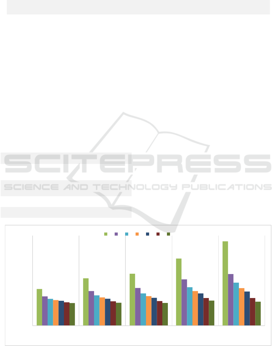
Table 2: Retailer's Demands.
Average
Uncertainty level (Standard
deviation)
Accuracy rate
(
)
Retailer
99%, 98%, 95%, 90%, and 80%
Retailer’s demand follows Gamma distribution
. Since the demands are non-stationary,
the parameters for Gamma distribution are
dependent on . According to the defined trends (
)
for the demand at each retailer,
and
take
different values.
In this paper first we do the experiment without
involving the entropy level, just to see how different
models behave, and then we add the entropy effect
(
) on safety stock calculation to check with the
results. Of course the results should be better, but we
measure whether the indicators are improved.
Table 3: Parameter values.
Notation
Parameter
values
Handling costs
25
Inventory holding costs per unit
per period
0.5
Travel costs for vehicle in Euro
per KM
1
Fix operating cost of vehicle
30
Average speed of vehicle
50
4 RESULTS AND DISCUSSIONS
The instances of DOE have been optimized and
simulated for 280 replications. The simulation model
generates gamma distributed demands according to
. The optimized results show the amount
of delivered product to the retailer in different
periods, together with inventory level at each period.
Also the costs to expect from this model. To verify
this, we simulated the DOE instances 280 times and
compared the results with the estimated outcome
from optimization model.
The indicators chosen in this paper show an
interesting move amongst different instances. Figure
1 displays the average inventory levels at the end of
the planning horizon for each instance. The
horizontal axis shows the accuracy rates of our data,
to see whether the inventory level changes if the
provided data is not accurate. As it is shown in this
figure, the level of inventory increases slightly
when the data accuracy is decreasing.
In addition, different considered safety stock
based model have different effects on the inventory
level. Model 9 (table 1) has the lowest inventory
while Model 1 has the highest volume. This
Figure 1: Inventory level.
0
20
40
60
80
100
120
140
160
180
99% 97% 95% 90% 80%
INVENTORY VOLUME
ACCURACY RATES
3 4 5 6 7 8 9
ICINCO 2019 - 16th International Conference on Informatics in Control, Automation and Robotics
662
difference is because of the safety stock reduction
policy in long term planning horizons. Moreover, the
difference between different models is the lowest
when the accuracy is 99%, meaning all models
behaving similar when the certainty of the demand
rate is the highest. By having low accuracy, the
models need to allocate more inventory to the
retailer and that results in high end inventory level.
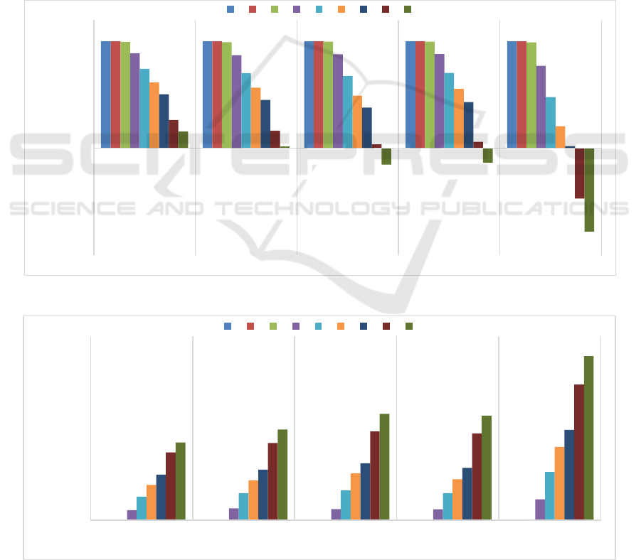
The other important indicator in this study is
inventory violation. This indicator shows the
percentage of having the retailer out of stock during
the whole planning horizon. These percentages are
shown in figure 2 for all the instances considered in
this paper. In this cases we pre-defined 10% of
inventory violation among the planning horizon, and
according to this, we check whether the actual stock-
out level varies in different instances.
The horizontal axis in figure 2 displays the
accuracy rates of different instances, while the
vertical axis shows the backlog percentage. As it is
shown in this figure, lack of accuracy in data results
in minor changes in IV levels. Even-though the
accuracy level is around 80%, still the models are
able to cover the demands for more than 82% in the
worst case (model 9), and 100% in the best cases
(model 1, 2, and 3). The trend in different accuracy
rates is the same. Model 1 is always with no stock-
out and model 9 with high stock-out level.
To have a better understanding of this indicator,
figure 3 presents the differences between expected
and actual level of backlog. Positive values
demonstrate the model satisfaction of the estimated
guaranteed service level and negative values show
the failure of the models to cover the estimated level
Figure 2: Service Level Accuracy.
Figure 3: Stock-out level.
-0.1
-0.08
-0.06
-0.04
-0.02
0
0.02
0.04
0.06
0.08
0.1
0.12
99% 97% 95% 90% 80%
SERVICE LEVEL DIFFERENCES
ACCURACY RATES
1 2 3 4 5 6 7 8 9
0
0.05
0.1
0.15
0.2
99% 97% 95% 90% 80%
BACKLOG PERCENTAGE
ACCURACY RATE
1 2 3 4 5 6 7 8 9
Inventory Routing Problem with Non-stationary Stochastic Demands
663
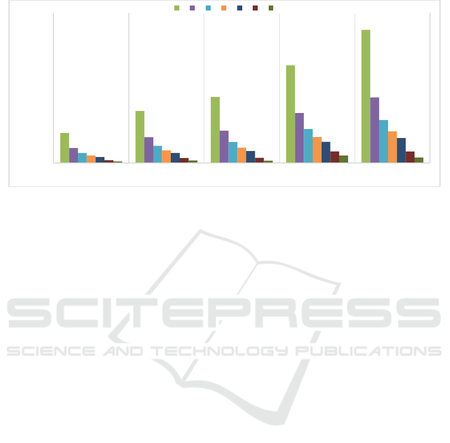
Figure 4: Inventory Accuracy.
of service. As it is clear, all the instances satisfied
the expected service except model 9 for the cases
with 95, 90, and 80 percent accuracy in data and
model 8 for the case with 80 percent accuracy in
data. This figure clarifies the ability of the proposed
models in satisfying the demands in different
situations. Even-though the amount of safety stock
decreases by the number of proposed models, still
they manage to have the expected service level.
From the other side this figure shows that in
most of the cases the actual level of service is more
than what was expected (more than 90 percent while
90% is enough), which means that the retailer keeps
extra level of inventory in most of the periods of
planning horizon to deal with the uncertainty in
demands. Therefore, having the bars more close to
zero in figure 3 shows the efficiency of the model
(in this case model 8) in satisfying the demand while
avoiding the huge inventory level.
To check with the models to see whether they are
accurate in their results, we compare the estimated
level of inventory at each period with actual levels.
Figure 4 illustrates this differences for all the
considered cases in this paper. Models with lower
level of safety stock are more accurate in the
inventory level in comparison with the ones with
bigger safety stock (we have excluded model 1 and 2
(table 1) in this figure due to the high level of
difference in inventory). In addition, the cases with
lower data accuracy have lower accuracy in their
results which makes sense, because the model needs
to compensate it with more delivered products which
might not be used in the end.
5 CONCLUSION
In this paper we considered stochastic demands in
IRP when the variability of demand increases among
the periods. Several uncertainty rates are examined
as well as different safety stock-based models to
solve the SPIRP model. We developed the SPIRP
model for one retailer with an average level of
demand, and standard deviation for each period. The
objective is to find an optimum level of safety stock
to be allocated to the retailer, in order to achieve the
expected level of service, and minimize the costs.
The performance of the model based on the defined
indicators and DOE cases is evaluated for a 50
period planning horizon, and simulated for 280
replications to compare the expected results with
actual outcomes.
The results have shown a gradual reduction in
inventory levels at the retailer for the cases with
smaller safety stock level. The models 7, 8, 9 (table
1) are almost the same regarding the inventory
volume and accuracy check, among all the defined
uncertainty levels. These models showed that for the
long term planning horizon we are able to reduce the
safety stock to minimize the costs. In addition, in
these models the impact of uncertainty level is less
than other models. Expected service level is
achieved in all the scenarios except for some cases
of model 9 and one case of model 8, due to the lack
of available inventory. For the future research, we
will involve more variation of cases in the design of
experiments to be able to evaluate the model from
different perspectives.
0
20
40
60
80
100
120
140
99%
97%
95%
90%
80%
INVENTORY ACCURACY
ACCURACY RATES
3 4 5 6 7 8 9
ICINCO 2019 - 16th International Conference on Informatics in Control, Automation and Robotics
664

REFERENCES
Abdul Rahim, M. K. I., Zhong, Y., Aghezzaf, E.-H. and
Aouam, T. (2014) Modelling and solving the
multiperiod inventory-routing problem with stochastic
stationary demand rates. International Journal of
Production Research, 52(14), 4351-4363.
Bertazzi, L., Bosco, A. and Laganà, D. (2015) Managing
stochastic demand in an Inventory Routing Problem
with transportation procurement. Omega, 56, 112-121.
Bertsimas, D., Brown, D. B. and Caramanis, C. (2011)
Theory and Applications of Robust Optimization.
SIAM Review, 53(3), 464-501.
Diaz, R., Bailey, M. P. and Kumar, S. (2016) Analyzing a
lost-sale stochastic inventory model with Markov-
modulated demands: A simulation-based optimization
study. Journal of Manufacturing Systems, 38, 1-12.
Manzini, R. and Bindi, F. (2009) Strategic design and
operational management optimization of a multi stage
physical distribution system. Transportation Research
Part E: Logistics and Transportation Review, 45(6),
915-936.
Pujawan, N., Arief, M. M., Tjahjono, B. and Kritchanchai,
D. (2015) An integrated shipment planning and
storage capacity decision under uncertainty A
simulation study. International Journal of Physical
Distribution and Logistics Management, 45(9-10),
913-937.
Purohit, A. K., Shankar, R., Dey, P. K. and Choudhary, A.
(2016) Non-stationary stochastic inventory lot-sizing
with emission and service level constraints in a carbon
cap-and-trade system. Journal of Cleaner Production,
113, 654-661.
Rahim, A. and Irwan, M. K. (2015) On the inventory
routing problem with stationary stochastic demand
rate. Ghent University.
Sagaert, Y. R., Aghezzaf, E.-H., Kourentzes, N. and
Desmet, B. (2018) Tactical sales forecasting using a
very large set of macroeconomic indicators. European
Journal of Operational Research, 264(2), 558-569.
Yadollahi, E., Aghezzaf, E. H. and Raa, B. (2017)
Managing inventory and service levels in a safety
stock‐based inventory routing system with stochastic
retailer demands. Applied Stochastic Models in
Business and Industry.
Inventory Routing Problem with Non-stationary Stochastic Demands
665
