
Computed Torque Control of an Aerial Manipulation System with a
Quadrotor and a 2-DOF Robotic Arm
Nebi Bulut
1
, Ali Emre Turgut
1
and Kutluk Bilge Arıkan
2
1
Department of Mechanical Engineering, Middle East Technical University, Çankaya, Ankara, Turkey
2
Department of Mechanical Engineering, TED University, Çankaya, Ankara, Turkey
Keywords: Aerial Manipulation, Computed Torque Control, Gain Optimization, Robotics, Quadrotor.
Abstract: This paper presents the control of an aerial manipulation system with a quadrotor and a 2-DOF robotic arm
by using the computed torque control method. The kinematic and dynamic model of the system is obtained
by modeling the quadrotor and the robotic arm as a unified system. Then, the equation of motion of the unified
system is got in the form of a standard robot dynamics equation. For the trajectory control of the system,
computed torque control is used. Gains of the controller are optimized by using nonlinear least squares method.
The performance and stability of the control structure are tested with a simulation case study.
1 INTRODUCTION
Unmanned air vehicles (UAVs) have already got the
attention of researchers from all around the world in
recent years. There are lots of researches have been
conducted. Especially, UAVs with rotary wing i.e.
quadrotors are the most studied ones (Kotarski,
Benic, and Krznar, 2016), (Das, Lewis, Subbarao,
2009), (Sadr, Moosavian, and Zarafshan, 2014), and
(Mahony, Kumar and Corke, 2012). There are certain
advantages of the quadrotors such as the ability of
vertical take-off and landing, staying hover position,
and capability of high agility and maneuverability. In
daily life, they are used for surveillance, rescue, and
filming.
These days, in order to increase capabilities of the
quadrotors, like carrying, painting and welding
operations, researches are conducted about aerial
manipulation. To obtain manipulated air vehicles, a
robotic arm is added to the bottom of these vehicles.
Different degrees of freedom serial robotic
manipulators that are attached to the UAVs are
studied (Kim, Choi, and Kim, 2013), (Caccavale,
Giglio, Muscio and Pierri, 2014), and (Jimenez-Cano,
Martin, Heredia, Ollero and Cano, 2013). Moreover,
aerial manipulation with parallel manipulators is
worked (Danko, Chaney and Oh, 2015). For
manipulation purposes, cable-suspended studies are
also available (Goodarzi, Lee and Lee, 2014),
(Sreenath, Kumar, 2013), and (Alothman, Guo and
Gu, 2017).
In literature, two main methods are followed to
model the unified quadrotor manipulator system. The
first approach is that kinematic and dynamic model of
the quadrotor is created, then behaving robotic arm as
a disturbance input to the quadrotor (Orsag, Korpela,
Bogdan and Oh, 2013) and (Khalifa and Fanni, 2017).
In the second method, quadrotor and robotic arm are
modeled as one system (Kim, Choi and Kim, 2013)
and (Caccavale, Giglio, Muscio and Pierri, 2014). For
controlling the unified system different approaches
have been developed. To deal with interaction forces
between end-effector of the robotic arm and the
environment, and disturbances, the compliance
control strategy is used (Giglio, and Pierri, 2014).
Also, a robust control strategy is studied for the
trajectory tracking control of the aerial manipulation
without effecting from the unmodelled dynamics and
uncertainties (Mello, Raffo and Adorno, 2016). For
the controller development, controller design stage
can be divided into in terms of whether a single
controller is designed or decoupled controllers are
designed to control the overall system. For the unified
system of robotic manipulator and quadrotor,
decoupled dynamics are used to development of
decoupled controller algorithms (Khalifa and Fanni,
2017). It can be seen that single controller
implementation is studied by exploiting coupled
equations of motion of the unified system (Kim, Choi
and Kim, 2013). The other aspect of the controller
design stage is whether a linear or nonlinear
controller has proceeded for the stable system
performance. A nonlinear model predictive controller
510
Bulut, N., Turgut, A. and Aríkan, K.
Computed Torque Control of an Aerial Manipulation System with a Quadrotor and a 2-DOF Robotic Arm.
DOI: 10.5220/0007965505100517
In Proceedings of the 16th International Conference on Informatics in Control, Automation and Robotics (ICINCO 2019), pages 510-517
ISBN: 978-989-758-380-3
Copyright
c
2019 by SCITEPRESS – Science and Technology Publications, Lda. All rights reserved
is studied to regulate the overall system around
optimized trajectories (Garimella and Kobilarov,
2015). Also, by using the feedback linearized
dynamics, linear controller (PID) implementations
are available (Khalifa and Fanni, 2017).
In this paper, Lagrange-D’Alembert formulation
is used to obtain the equation of motion of the unified
system in the form of standard robotics equations of
motion. For controlling the unified system, computed
torque control with PID outer loop is designed. For
the gain optimization procedure, multi-objective
nonlinear least square solver of Matlab Global
Optimization Toolbox is used. The ITAE (The
Integral of Time multiply Absolute Error) is selected
as an objective function to minimize the error
between the input and the output. For simulating more
realistic scenario, experimentally identified
quadrotor’s dc motors’ transfer function and second
order torque filtering transfer function for the robotic
arm is implemented in the system’s simulation.
This paper is organized in 5 sections. Section 1 is
the introduction to this paper. Section 2 includes
details about the modeling of the unified system.
Section 3 consists of controller design pattern.
Simulation results are presented in section 4. Finally,
the discussion and conclusion of this paper take part
in section 5.
2 MODELLING
2.1 Kinematics
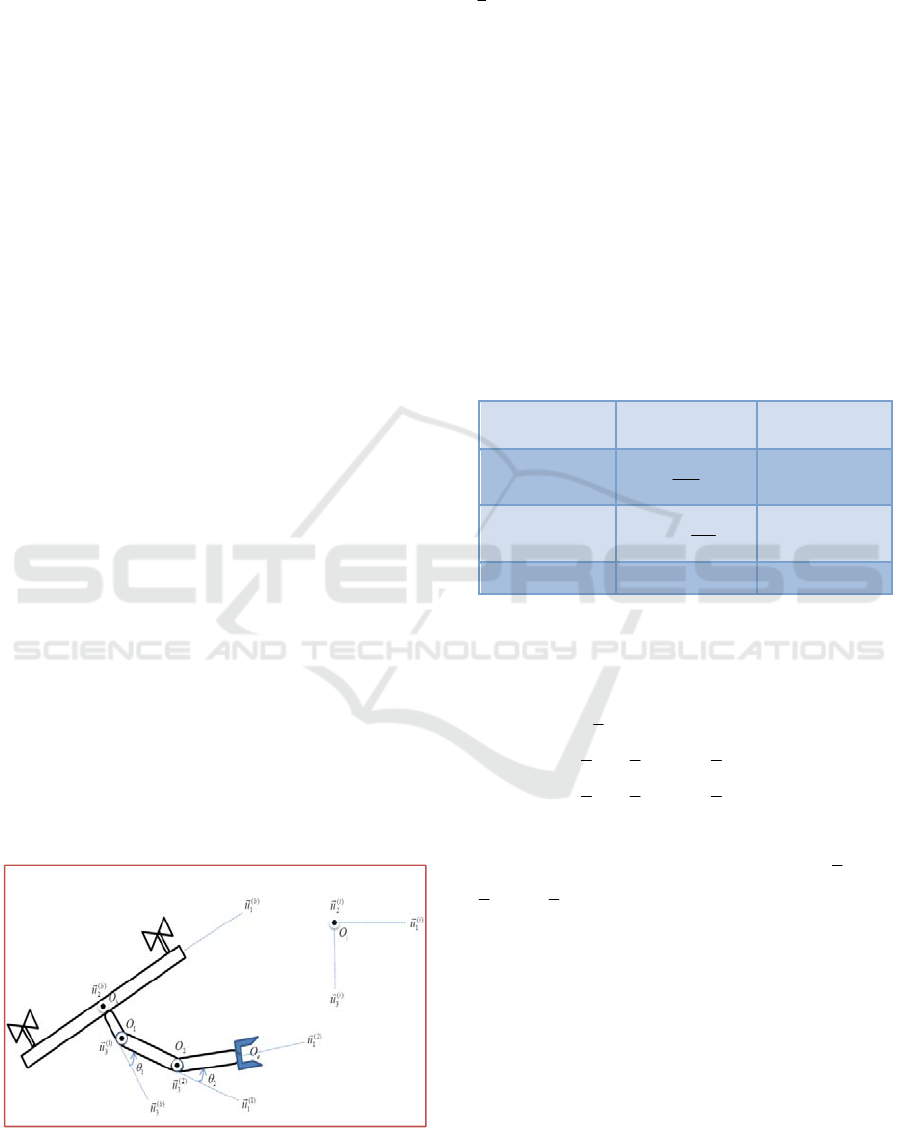
Some of the kinematic parameters of the unified
system can be seen in Figure 1. In this figure,
i
O
,
b
O
,
1
O
,
2
O
and
e
O
are the origins of the reference frames
of the inertial, quadrotor’s body, link-1, link-2 and the
end-effector of the robot arm, respectively.
Figure 1: Side view of the unified system and some of the
kinematic parameters.
Orientation of the quadrotor is designated by the
set of Euler angles that are roll, pitch and yaw angles,
T
. Their names are phi, theta, and psi in
the Latin Alphabet. By using these angles, the
transformation matrix from the quadrotor’s body-
fixed reference frame to the earth-fixed reference
frame can be written as follows,
(,)
ˆ
ib
cc css sc csc ss
Cscsssccssccs
scs cc
(1)
In Eq. (1),
s
and
c
are used in place of sin
and
cos
. The table that consists of Denavit–Hartenberg
parameters for the robotic arm can be given as below.
Where,
k
is twist angle,
k
is joint angle, and
k
b
is
the offset between the joints.
Table 1: Denavit–Hartenberg Parameters.
Parameters
Link-1
Link-2
k
2
0
k
1
3
2
2
k
b
1
b
2
b
Position of the center of the mass of the quadrotor,
link-1 and link-2 of the robotic arm with respect to the
inertial fixed reference frame can be written as
follows,
()
T
i
q
pxyz
(2)
() () (,) ( )
11
ˆ
iiibb
q
ppCp
(3)
() () (,) ( )
22
ˆ
iiibb
q
ppCp
(4)
In these equations, x, y and z are Cartesian
coordinates of the position of the quadrotor,
()i
q
p
, and
()
1
b
p
and
()
2
b
p
are the positions of the link-1 and link-2
in body fixed reference frame of the quadrotor.
The matrix that defines the relationship between
the angular velocity of the quadrotor and time
derivative of the Euler angles,
ˆ
L
.
10
ˆ
0
0
s
L
ccs
s
cc
(5)
Computed Torque Control of an Aerial Manipulation System with a Quadrotor and a 2-DOF Robotic Arm
511

Then, the relation can be further written as by
noticing that
()b
q
w
is the angular velocity of the
quadrotor in body fixed reference frame,
()
ˆ
b
q
wL
(6)
Also, further relations can be given as,
() (,) ( )
ˆ
iibb
qq
wCw
(7)
() (,)
ˆ
ˆˆ
iib
q
wCLT
(8)
Where,
()i
q
w
is the angular velocity in the inertial
fixed reference frame, and
ˆ
T
maps the rate of change
of the Euler angles into
()i
q
w
. Overhead dot is used for
the time derivative of the corresponding parameter.
Jacobian matrix, J can be used to express the
linear and angular velocities of the link-1 and link-2
in quadrotor’s body fixed reference frame as,
()
11
ˆ
b
v
pJ
(9)
()
22
ˆ
b
v
pJ
(10)
()
11
ˆ
b
w
wJ
(11)
()
22
ˆ
b
w
wJ
(12)
Then, linear and angular velocities in the inertial
fixed reference frame can be written as,
() () (,) ( ) (,) ( )
111
ˆˆ
iiibbibb
q
p p Cp Cp
(13)
() () (,) ( ) (,) ( )
222
ˆˆ
iiibbibb
q
p p Cp Cp
(14)
() () ( ) (,) ( ) (,)
111
ˆˆ
ˆ
()
ii bibbib
qq v
ppSSMwCpCJ
(15)
() () ( ) (,) ( ) (,)
222
ˆˆ
ˆ
()
ii bibbib
qq v
ppSSMwCpCJ
(16)
() () (,)
11
ˆ
ˆ
iiib
qw
wwCJ
(17)
() () (,)
22
ˆ
ˆ
iiib
qw
wwCJ
(18)
SSM is used for skew-symmetric operation.
Generalized coordinates and velocities of the unified
system can be defined as,
12
12
T
T
qxyz
qxyz
(19)
By using linear and angular velocity influence
coefficients,
ˆ
V
and
ˆ
W
, respectively, and Eq. (19),
the linear and angular velocities can be written further
as (Ozgoren, 2017),
()
33 35
ˆ
ˆˆ
0
i
qxx q
pI qVq
(20)
()
33 32
ˆˆ
ˆˆ
00
i
qx x q
wTqWq
(21)
() (,) ( ) (,)
133 1 1 1
ˆˆ
ˆˆˆˆ
()
iibbib
xv
pI SSMCpTCJqVq
(22)
() (,) ( ) (,)
233 2 2 2
ˆˆ
ˆˆˆˆ
()
iibbib
xv
p I SSM C p T C J q V q
(23)
() (,)
133 1 1
ˆˆ
ˆˆ ˆ
0
iib
xw
wTCJqWq
(24)
() (,)
233 2 2
ˆˆ
ˆˆ ˆ
0
iib
xw
wTCJqWq
(25)
2.2 Dynamics
Equation of motion of the unified system is obtained
by using the following form of the Lagrange-
D’Alembert formulation.
()
ext
dL L
uu
dt q q
LKU
(26)
In Eq. (26), K is the total kinetic energy and U is
the total potential energy of the unified system, and L
is the Lagrange operator. Also,
u and
ext
u
are the
generalized input force and interaction force between
end-effector and the environment, respectively.
2.2.1 Kinetic and Potential Energies
The total kinetic energy of the overall system is the
sum of the kinetic energies of the quadrotor body with
mass
b
m
, link-1 with mass
1
m
, and link-2 with mass
2
m
.
12b
K
KKK
(27)
,,
() ()() ()
11
ˆ
ˆˆ
22
ib ibT
iT i
bbq
iT i
qq b q
Km CICpp
(28)
,,1 ,1,
() ()
111 1 1
() ()
11
ˆˆ
11
ˆ
22
ˆˆ
ib b
iT
bTibT
iT ii
Km CCIpCCp
(29)
,,2 ,2,
() ()
2
() (
2222
)
22
ˆˆ
11
ˆ
22
ˆˆ
ib b
iT
bTibT
iT ii
Km CCIpCCp
(30)
In the above equations,
I
is the constant inertia
matrix in the corresponding body fixed reference
frames.
Similarly, potential energies of each mass
elements as follows,
12b
UU UU
(31)
()
3
ti
bb q
Umgup
(32)
()
1131
ti
Umgup
(33)
()
3222
ti
Umgup
(34)
ICINCO 2019 - 16th International Conference on Informatics in Control, Automation and Robotics
512

In these equations,
g
is the gravity.
2.2.2 Equation of Motion
By plugging Eq. (31) and Eq. (27) into Eq. (26),
following equation of motion of the unified system is
obtained.
ˆ
ˆ
() (,) ()
ext
M
qq Cqqq Gq u u
(35)
In above equation,
ˆ
M
is the positive definite
inertia matrix,
ˆ
C
includes centripetal, Coriolis and
gyroscopic terms, and gravity terms take part in
matrix
ˆ
G
. To calculate inertia matrix, following
kinetic energy formulation is used (Siciliano,
Sciavicco, Villani and Oriolo, 2009).
1
ˆ
()
2
T
K
qMqq
(36)
Inertia matrix can be further written by using Eq.
(36) and from Eq. (20) to Eq. (25) as
(,) (,)
2
(,) ( ,) (,) ( , )
1
ˆˆ
ˆˆˆˆˆˆ
()
ˆˆ ˆˆ
ˆˆˆ ˆ ˆ
()()
T T ib ibT
qbq q b q
TTibbkibbkT
kkk k k k
k
Mq VmV WC IC W
VmV W C C I C C W
(37)
Also, elements of the
ˆ
C
can be calculated by using
following relation (Siciliano, Sciavicco, Villani and
Oriolo, 2009),
8
,,
,
,
1
1
2
aj jb
ab
ab
j
jba
mm
m
c
qqq
(38)
Finally, the column matrix
ˆ
G
is given as,
ˆ
()
U
Gq
q
(39)
Generalized input force,
u and interaction force
that is applied on the tip point of the end-effector,
ext
u
are obtained by using virtual work principle.
()
()
12
ˆ
b
q
b
q
f
uH
(40)
(,)
()
33 32
()
33 32
12
23 23 22
ˆˆˆ
00
ˆˆ
ˆ
00
ˆˆ
ˆ
00
ib
b
xx
q
tb
xxq
xxx
C
f
uL
I
(41)
33 33
()
33
ˆ
ˆ
0
ˆ
()
ˆˆ
xx
b
ext e x
TT
ve we
I
uSSMpI
JJ
P
(42)
In Eq. (40),
ˆ
det( ) cos( )
H
(43)
Therefore, if
2
n
, nZ ,
Then,
ˆ
H
is an invertible square matrix. In this study,
this condition is satisfied.
Where *x* is used to show sizes of matrices.
()b
e
p
is the position of the end-effector’s tip point in the
quadrotor’s body-fixed reference frame. Also,
ˆ
J
is
the Jacobion matrix of the end-effector. Forces and
torques that are generated by the quadrotor’s dc
motors are
()b
q
f
and
()b
q
, respectively. In addition to
that, the generated torques by the arm joints are
12
.
Moreover,
P
is the column matrix of applied forces
and moments on the end-effector’s tip point.
()
00
T
b
qz
f
f ,
()
123
T
b
qqqq
(44)
123 1 2 3
T
PFFFMMM
(45)
Relationship between quadrotor’s dc motors
rotational speed and the generated force and torques
by the quadrotor’s motor are written in Eq. (46).
Where
T
c
and
Q
c
are dc motor’s thrust and drag
coefficients.
2
1
2
1
2
2
2
3
2
3
4
00
00
zTTTT
qTT
qT T
qQQQQ
fcccc
dc dc
dc dc
cc cc
(46)
Where,
z
f
is the sum of the total thrust generated by
the quadrotor’s rotors.
For the transfer function between commanded
rotational speed of the quadrotor’s dc motor and
achieved rotational speed, following transfer function
that is obtained by the Yıldız, 2015 is used.
_
_0.98
()
_
_0.0621
Achieved Rotor Speed
Gs
Commanded Rotor Speed s
(47)
It is assumed that arm joints’ servo motors are
getting torque input from the controller. Instead of
directly applying the controller torque inputs to the
joints, commanded torques are filtering by using a
Computed Torque Control of an Aerial Manipulation System with a Quadrotor and a 2-DOF Robotic Arm
513
second order filter in the following form with
0.707
and
20
n
w
Hz.
2
22
()
2
n
nn
w
Gs
s
ws w
(48)
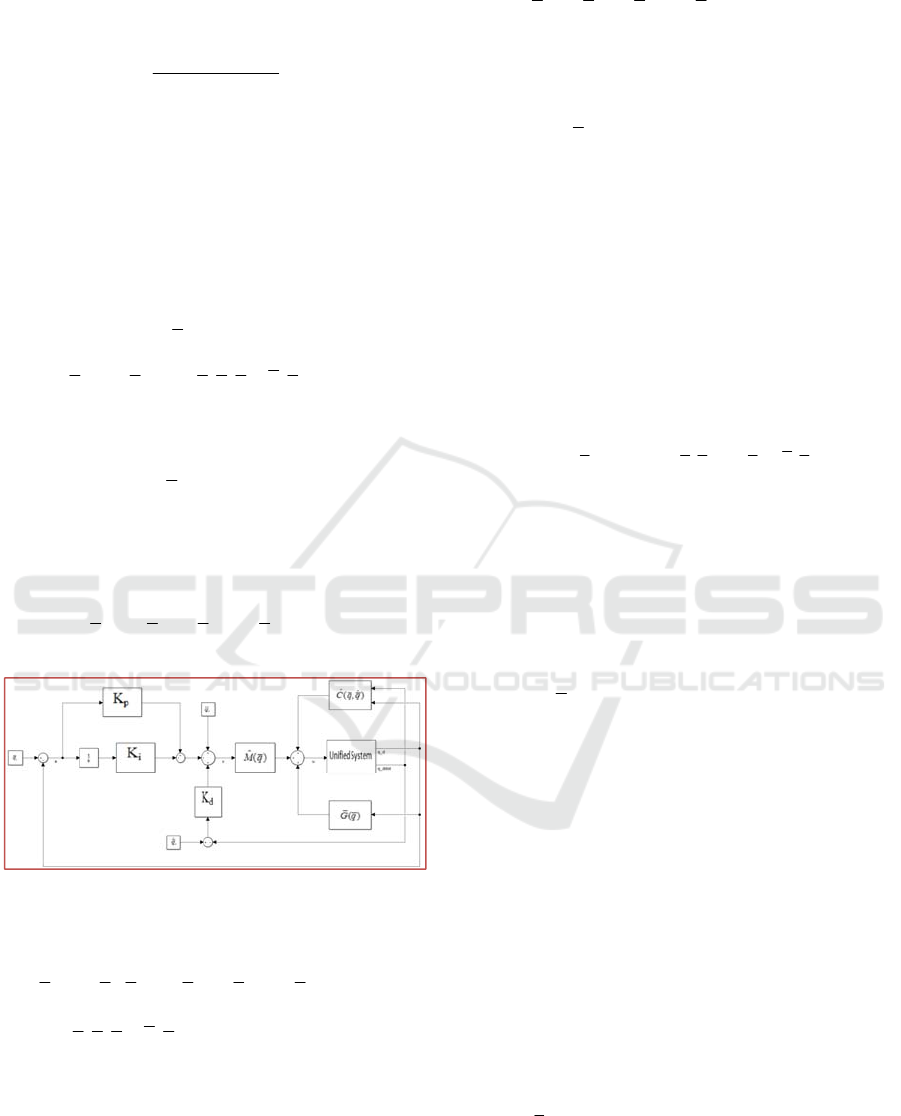
3 CONTROLLER DESIGN
To control the overall system, computed torque
control with PID outer loop is designed. Control
architecture of the unified system can be seen in
Figure 2.
Following control input is selected to control the
overall system while
0
ext
u
.
ˆ
ˆ
() (,) ()
u Mqv Cqqq Gq
(49)
Then, substituting this control law into Eq. (35), it
follows that,
qv
(50)
After this control input, complicated nonlinear
controller design turns into a simpler design problem.
Then,
v
can be selected as,
0
ˆ
()
ˆ
dp d
t
i
K
edvq KeKe
(51)
Figure 2: Control architecture of the overall system.
Hence, the overall control input is written as,
0
ˆˆˆ
()( )
ˆ
(,
(
)()
)
dp
t
id
KeuMqq dKe Ke
Cqqq Gq
(52)
Where
ˆ
p
K
,
ˆ
d
K
and
ˆ
i
K
are the positive definite
diagonal gain matrices.
Then, the resulting error dynamics can be written
as,
0
ˆ
)0
ˆ
(
pd
t
i
KeKe dKe e
(53)
According to linear system theory, convergence of
the tracking error to zero is guaranteed (Siciliano and
Khatib, 2008).
Note 1:
d
q
can be calculated numerically, but it
causes derivative noises. In simulations it is assumed
to be zero.
3.1 Quadrotor Position Control
Bu using Eq. (49), to control the quadrotor’s position
following expression can be written. In this equation,
subscripts are used to show the corresponding indices
of the matrices. However, Eq. (54) requires the
desired roll and pitch angles. In this stage, they are
not available.
(1:3,1:8)
1
2(1:3,1:8) (1:3)
3
ˆ
ˆ
[()] [(,)] [()]
u
uMq vCqqqGq
u
(54)
To cope with this problem, following modified
form of the inertia matrix is used.
***00***
***00***
***00***
********
ˆ
()
********
********
********
********
Mq
(55)
First three elements of the columns four and five
are replaced by the zero. By this way, the requirement
of the knowledge of the desired roll and pitch angles
is eliminated. These elements of the inertia matrix are
often negligible since robotic arm’s links are much
lighter than quadrotor’s body (Arleo, Caccavale,
Muscio and Pierri, 2013).
Then, to compute desired roll and pitch angles,
from Eq. (41) and Eq. (44) following relation can be
written
1
123 2
3
()
()
()
z
z
z
ucscssf
uu ssccsf
uccf
(56)
From Eq. (56)
ICINCO 2019 - 16th International Conference on Informatics in Control, Automation and Robotics
514
123 123
T
z
f
uu
(57)
12
3
cos( ) sin( )
arctan( )
des
uu
u
(58)
12
sin( ) cos( )
arcsin( )
des
z
uu
f
(59)
3.2 Quadrotor Attitude Control
From Eq. (49), following relation can be written
(4:6,1:8)
4
456 5 (4:6,1:8) (4:6)
6
ˆ
ˆ
[()] [(,)] [()]
u
uuMqvCqqqGq
u
(60)
Eq. (41) and Eq. (60) give the torques of the
vehicle as,
() 1
456
ˆ
()
bt
q
Lu
(61)
Note 2 : Quadrotor inputs that are angular speeds
of the dc motors can be computed by benefiting from
the Eq. (46), Eq. (44), Eq. (57) and Eq. (61).
3.3 Manipulator Joint Angles Control
From Eq. (49),
( 7:8 ,1:8 )
7
78 ( 7:8 ,1:8 ) ( 7:8)
8
ˆ
ˆ
[()] [(,)] [()]
u
uMqvCqqqGq
u
(62)
Eq. (41) and Eq. (62) give the torque inputs of the
arm joints as,
12 78
u
(63)
3.4 Gain Optimization
Gains of the computed torque controller are
optimized by using nonlinear least-squares solver of
the MATLAB Global Optimization Toolbox. For the
objective function, ITAE (The Integral of Time
multiply Absolute Error) given in Eq. (64) is used.
0
()
T
I
TAE t e t dt
(64)
This is a multi-objective optimization problem
since there are 8 trajectories that should be optimized
at the same time.
To make the optimization faster, Simulink model
of the overall system is transformed into executable
model and then, gains are tuned for the minimum
trajectory errors.
4 SIMULATION RESULTS
Proposed control algorithms are tested by simulation
in Matlab/Simulink environment. Table 2 shows
numerical values that are used in the simulation.
Table 2: Numeric Parameters of the Unified System.
Quadrotor Link-1 & Link-2
Mass (kg)
2.6550 0.1700
d (m)
0.6870 0.3000
I
xx
(kgm
2
)
0.0457 7.0830e-05
I
yy
(kgm
2
)
0.0457 0.0013
I
zz
(kgm
2
)
0.0846 0.0013
Table 3: Simulation Scenario Parameters.
Time(s) 0-9 10-19 20-25 25-60
x
(m)
0-5 5 5 5
y (m)
0-3 3 3 3
z
(m)
0-(-2) -2 -2 -2
(deg)
- - - -
(deg)
- - - -
(deg)
0 0 0 0
1
(deg)
0 0-15 15 15
2
(deg)
0 0-10 10 10
1
F
(N)
0 0 0-5 5
2
F
(N)
0 0 0-1 1
3
F
(N)
0 0 0-5 5
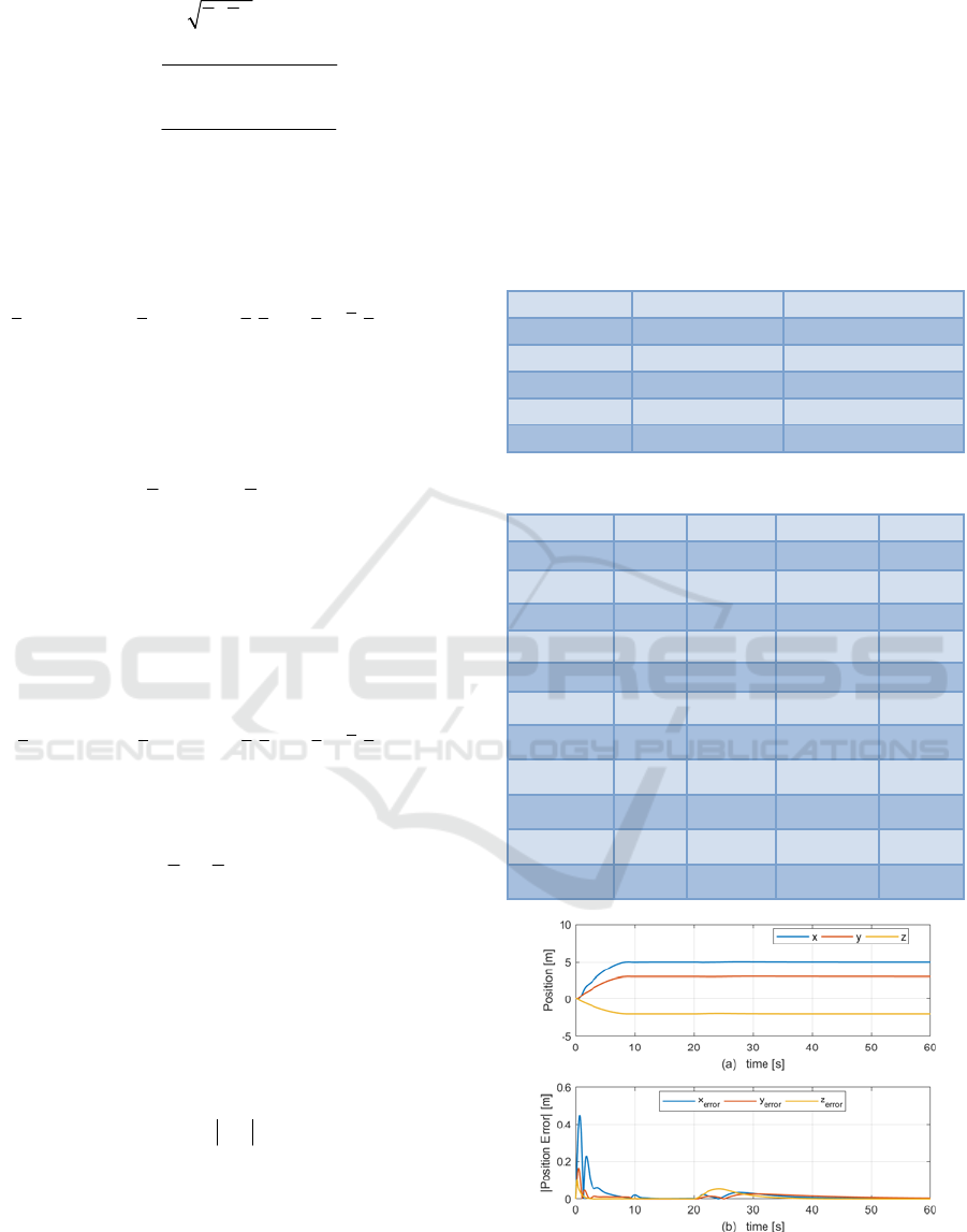
Figure 3: (a): Position of the quadrotor, (b): Absolute
position error of the quadrotor.
Computed Torque Control of an Aerial Manipulation System with a Quadrotor and a 2-DOF Robotic Arm
515
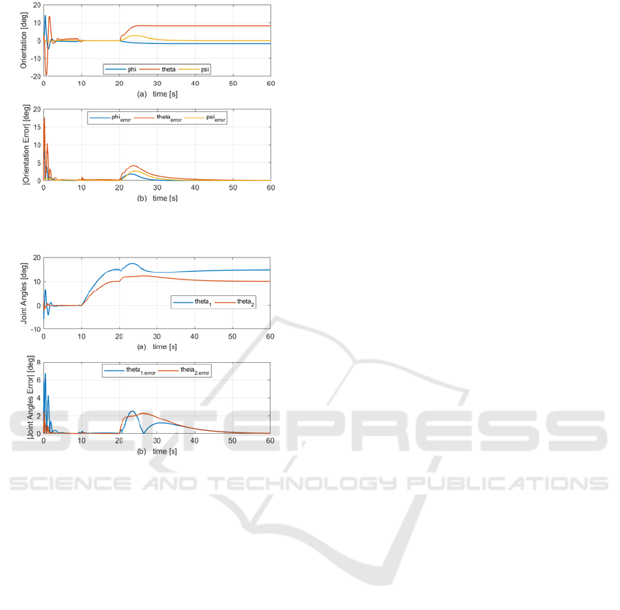
Figure 4: (a): Orientation of the quadrotor, (b): Absolute
orientation error of the quadrotor.
Figure 5: (a): Angular position of the joints of the robotic
arm, (b): Absolute angular position error of the joints of the
robotic arm.
Table 3 shows the simulated scenario parameters.
From 0 to 9 seconds quadrotor positions x, y and z are
commanded, and then, they are held constant through
the simulation, other parameters are held as zero. Roll
and pitch angles are the intermediate control inputs,
and they are not directly controlled. From 10 to 19
seconds 15 degree and 10 degree joint angles are
commanded to the robotic arm, and then they are
commanded to stay in these angles. From 20 to 25
seconds interaction forces are applied to the tip point
of the end-effector, and then they stay constant to the
end of the simulation.
Figure 3 shows the achieved quadrotor position in
3-D space and the error between the desired and the
achieved position. Euler angles of the quadrotor and
the error between the commanded and actual Euler
angles are demonstrated in Figure 4. Finally, the
angular position of the robotic arm joints and the error
between the desired and achieved joint angles are
given in Figure 5.
5 DISCUSSION AND
CONCLUSION
In this paper, an aerial manipulation system
consisting of a quadrotor and a robotic arm is studied.
Equation of motion of the unified system is obtained
in the form of equations of standard robotic systems.
Then, the computed torque controller is designed for
the trajectory tracking. Gains of the controller is
optimized based on minimizing the error between the
input and the output states of the robotic system. The
designed controller is tested in the simulation
environment with the highly nonlinear dynamic
model of the system in addition to quadrotor’s dc
motors’ transfer functions and torque filters of the
robot arm’s joints.
From Figure 3, quadrotor is commanded to come
to desired positions in 9 seconds. Then, the robotic
arm is moved from 10-19 seconds to the desired
position. This movement does not affect the position
of the quadrotor too much. However, from 20 to 25
seconds, interaction forces are applied from the
starting from the zero value and continue to apply to
the end of the simulation. As a result, positions of the
quadrotor are affected by the interaction forces, but
the controller shows a robust behavior and brings the
quadrotor to its original position. While doing this, to
balance the interaction forces, quadrotor tilts and has
nonzero roll and pitch angles as seen from Figure 4
starting from time = 20 seconds. This is an expected
behavior since quadrotor is an underactuated vehicle,
and x and y positions are coupled with the pitch and
roll angles, respectively. Angular positions of the
robotic arm also disturbed by the interaction forces.
However, due to the controller action, joint angles
settle down to their original values.
Simulation studies shows that proposed controller
can achieve good trajectory tracking performance for
all states, simultaneously. Also, under the action of
interaction forces, it can deal with these disturbances
up to some points.
REFERENCES
Kotarski, D., Benic, Z., Krznar, M., 2016. Control Design
for Unmanned Aerial Vehicles with Four Rotors.
Interdisciplinary Description of Complex Systems 14,
236–245.
Das, A., Lewis, F., Subbarao, K., 2009. Dynamic inversion
with zero-dynamics stabilisation for quadrotor control.
IET Control Theory & Applications 3, 303–314.
ICINCO 2019 - 16th International Conference on Informatics in Control, Automation and Robotics
516

Sadr, S., Moosavian, S. A. A., Zarafshan, P., 2014.
Dynamics Modeling and Control of a Quadrotor with
Swing Load. Journal of Robotics 2014, 1–12.
Mahony, R., Kumar, V., Corke, P., 2012. Multirotor Aerial
Vehicles: Modeling, Estimation, and Control of
Quadrotor. IEEE Robotics & Automation Magazine 19,
20–32.
Goodarzi, F. A., Lee, D., Lee, T., 2014. Geometric
stabilization of a quadrotor UAV with a payload
connected by flexible cable. 2014 American Control
Conference.
Sreenath, K., Kumar, V., 2013. Dynamics, Control and
Planning for Cooperative Manipulation of Payloads
Suspended by Cables from Multiple Quadrotor Robots.
Robotics: Science and Systems IX.
Alothman, Y., Guo, M., Gu, D., 2017. Using iterative LQR
to control two quadrotors transporting a cable-
suspended load. IFAC-PapersOnLine 50, 4324–4329.
Kim, S., Choi, S., Kim, H. J., 2013. Aerial manipulation
using a quadrotor with a two DOF robotic arm. 2013
IEEE/RSJ International Conference on Intelligent
Robots and Systems.
Caccavale, F., Giglio, G., Muscio, G., Pierri, F., 2014.
Adaptive control for UAVs equipped with a robotic
arm. IFAC Proceedings Volumes 47, 11049–11054.
Jimenez-Cano, A., Martin, J., Heredia, G., Ollero, A., Cano,
R., 2013. Control of an aerial robot with multi-link arm
for assembly tasks. 2013 IEEE International
Conference on Robotics and Automation.
Danko, T. W., Chaney, K. P., Oh, P. Y., 2015. A parallel
manipulator for mobile manipulating UAVs. 2015
IEEE International Conference on Technologies for
Practical Robot Applications (TePRA).
Orsag, M., Korpela, C., Bogdan, S., Oh, P., 2013. Lyapunov
based model reference adaptive control for aerial
manipulation. 2013 International Conference on
Unmanned Aircraft Systems (ICUAS).
Khalifa, A., Fanni, M., 2017. A new quadrotor
manipulation system: Modeling and point-to-point task
space control. International Journal of Control,
Automation and Systems 15, 1434–1446.
Giglio, G., Pierri, F., 2014. Selective compliance control for
an unmanned aerial vehicle with a robotic arm. 22nd
Mediterranean Conference on Control and Automation.
Mello, L. S., Raffo, G. V., Adorno, B. V., 2016. Robust
whole-body control of an unmanned aerial manipulator.
2016 European Control Conference (ECC).
Garimella, G., Kobilarov, M., 2015. Towards model-
predictive control for aerial pick-and-place. 2015 IEEE
International Conference on Robotics and Automation
(ICRA).
Ozgoren, M. K., 2017. Lecture Notes for ME 522
(Principles of Robotics), Department of Mechanical
Engineering, METU.
Siciliano, B., Sciavicco, L., Villani, L., Oriolo, G., 2009.
Robotics Modelling, Planning and Control. Springer,
London.
Yıldız, M., 2015. Effects Of Active Landing Gear On The
Attitude Dynamics Of A Quadrotor (thesis). Ankara.
Siciliano, B., Khatib, O., 2008. Springer handbook of
robotics: Springer-Verlag, New York Inc.
Arleo, G., Caccavale, F., Muscio, G., Pierri, F., 2013.
Control of quadrotor aerial vehicles equipped with a
robotic arm. 21st Mediterranean Conference on Control
and Automation.
Lewis, F. L., Abdallah, C. T., Dawson, D. M., Lewis, F. L.,
2018. Robot manipulator control: theory and practice.
Lightning Source UK Ltd., Milton Keynes UK.
Computed Torque Control of an Aerial Manipulation System with a Quadrotor and a 2-DOF Robotic Arm
517
